Content
Introduction
Artificial Neuron
Weighted Sum for Pre-Activation Value
ReLU Activation Function for Post-Activation
Bias Term
S-Shaped Functions – TANH and SIGMOID
Network Impact
Summary
References
Introduction
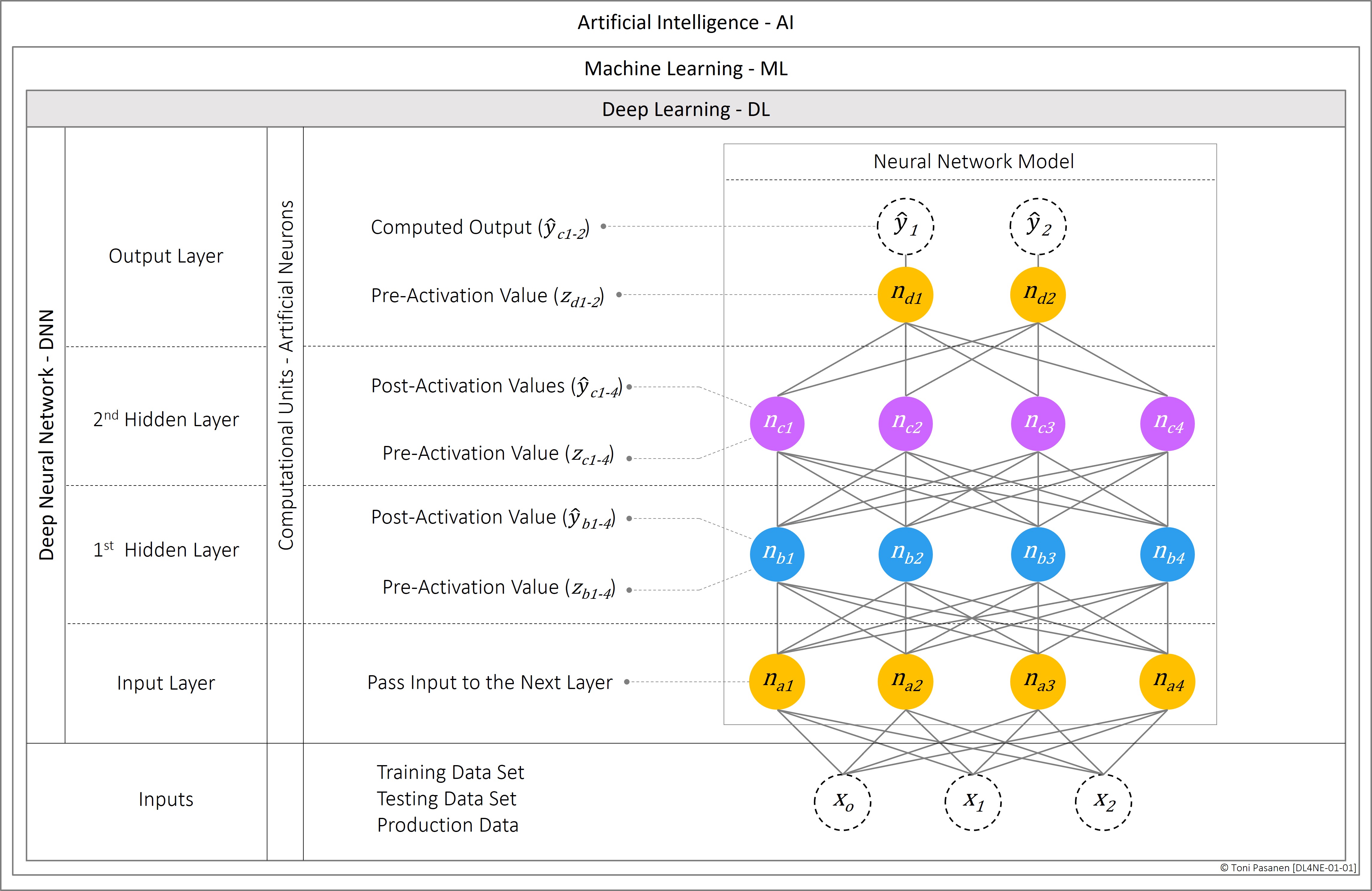
Artificial Intelligence (AI) is a broad term for solutions that aim to mimic the functions of the human brain. Machine Learning (ML), in turn, is a subset of AI, suitable for tasks like simple pattern recognition and prediction. Deep Learning (DL), the focus of this section, is a subset of ML that leverages algorithms to extract meaningful patterns from data. Unlike ML, DL does not necessarily require human intervention, such as providing structured, labeled datasets (e.g., 1,000 bird images labeled as “bird” and 1,000 cat images labeled as “cat”).
DL utilizes layered, hierarchical Deep Neural Networks (DNNs), where hidden and output layers consist of computational units, artificial neurons, which individually process input data. The nodes in the input layer pass the input data to the first hidden layer without performing any computations, which is why they are not considered neurons or computational units. Each neuron calculates a pre-activation value (z) based on the input received from the previous layer and then applies an activation function to this value, producing a post-activation output (ŷ) value. There are various DNN models, such as Feed-Forward Neural Networks (FNN), Convolutional Neural Networks (CNN), and Recurrent Neural Networks (RNN), each designed for different use cases. For example, FNNs are suitable for simple, structured tasks like handwritten digit recognition using the MNIST dataset [1], CNNs are effective for larger image recognition tasks such as with the CIFAR-10 dataset [2], and RNNs are commonly used for time-series forecasting, like predicting future sales based on historical sales data.
To provide accurate predictions based on input data, neural networks are trained using labeled datasets. The MNIST (Modified National Institute of Standards and Technology) dataset [1] contains 60,000 training and 10,000 test images of handwritten digits (grayscale, 28x28 pixels). The CIFAR-10 [2] dataset consists of 60,000 color images (32x32 pixels), with 50,000 training images and 10,000 test images, divided into 10 classes. The CIFAR-100 dataset [3], as the name implies, has 100 image classes, with each class containing 600 images (500 training and 100 test images per class). Once the test results reach the desired level, the neural network can be deployed to production.
Figure 1-1: Deep Learning Introduction.
Artificial Neuron
As we saw in the previous section, DNNs leverage a hierarchical, layered, role-based (input layer, n hidden layers, and output layer) network model, where each layer consists of artificial neurons. Neurons in different layers may be fully or partially connected to neurons in the other layers, depending on the DNN’s network model. However, neurons within the same layer are not connected.
The logical structure and functionality of an artificial neuron aim to emulate those of a biological neuron. A biological neuron transmits electrical signals to its peer neuron via the output axon to the axon terminal, which connects to the dendrites of the peer neuron at a connection point called a synapse. A biological neuron may receive signals from multiple dendrites, and if the signal is strong enough, it activates the neuron, causing the cell body to trigger a signal through its output axon, which connects to another neuron, and the process continues.
An artificial neuron, as a computational unit, calculates the weighted sum (z = pre-activation value) of the input (x) received from the previous layer, adds a bias value (b), and applies an activation function to produce the output (ŷ = post-activation value).
The weight value for the input can be loosely compared to a synapse since it represents a connection, input values are assigned with weight. The weights-to-neuron association, in turn, can be seen as analogous to dendrites. The computational processes (weighted sum of inputs, bias addition, and activation functions) represent the cell body, while the connections to other neurons can be compared to output axons. In Figure 1-2, bn refers to a biological neuron. From now on, "neuron" will refer to an artificial neuron.
Figure 1-2: Construct of an Artificial Neuron.
Weighted Sum for Pre-Activation Value
The lower part of Figure 1-2 depicts the mathematical formulas of a neuron. The pre-activation value z is the weighted sum of the inputs. Although the bias is not part of the input data, a neuron treats it as an input variable when calculating the weighted sum. Each input x has a corresponding weight w. The calculation process is straightforward: each input value is multiplied by its corresponding weight, and the results are summed to obtain the weighted sum z.
The capital Greek letter sigma ∑ in the formula indicates that we are summing a series of terms, which, in this case, are the input values multiplied by their respective weights. The letter n specifies how many terms are being summed (four pairs of inputs and weights), while the letter iii denotes the starting point of the summation (bias b0 and weight w0). The equation for the weighted sum is:
z = b0w0 + x1w1 + x2w2 + x3w3.
ReLU Activation Function for Post-Activation
Next, the process applies an activation function, ReLU (Rectified Linear Unit) [4] in our example, to the weighted sum z obtain the post-activation value ŷ. The output of the ReLU function is z if z is greater than zero (0); otherwise, the result is zero (0). This can be written as:
ŷ = MAX (0, z)
which selects the larger value between 0 and variable z. The figure 1-3 depicts the ReLU activation function.
Figure 1-3: Construct of an Artificial Neuron.
Based on the figure 1-3 we can use the mathematical definition below for ReLU:
Bias Term
In the example calculation above, imagine that all input values are zero. Without a bias term, the activation value will be zero, regardless of how large the weight parameters are. Therefore, the bias term allows the neuron to produce non-zero outputs, even when all input values are zero.
S-Shaped Functions – TANH and SIGMOID
The ReLU function is a non-linear activation function. Naturally, there are other activation functions as well. The Hyperbolic Tangent (tanh) [5] and the logistic Sigmoid [6] functions are examples of S-shaped functions that are symmetric around zero. Figure 1-4 illustrates that as the positive z value increases, the tanh function approaches one (1), while as the negative z value decreases, it approaches -1. Thus, the range of the tanh function is from -1 to 1. Similarly, the sigmoid function's S-curve is also symmetric around zero, but its range is from 0 to 1.

Figure 1-4: Tanh and Sigmoid functions.
Here are examples of both functions using the same pre-activation value of 3.02, as in the ReLU activation function example.
Note, the ⅇ represents Euler’s Number ⅇ≈ 2.718. The symbol σ represents the sigmoid function.
The formula for tanh function is:
The tanh function for z = 3,02
The formula for sigmoid function is:
The sigmoid function for z = 3,02
The symbol σ represents sigmoid function.
For z=3.02, both the sigmoid and tanh functions return values close to 1, but the tanh function is slightly higher, approaching its maximum of 1 more quickly than the sigmoid.
Which activation function should we use? The ReLU function has largely replaced the tanh and sigmoid functions due to its simplicity, which reduces the required computation cycles. However, if tanh and sigmoid are used, tanh is typically applied in the hidden layers, while sigmoid is used in the output layer.
Network Impact
A single artificial neuron is the smallest unit of a neural network. The size of the neuron depends on its connections to input nodes. Every connection has an associated weight parameter, which is typically a 32-bit value. In our example, with 4 connections, the size of the neuron is 4 x 32 bits = 128 bits.
Although we haven’t defined the size of the input in this example, let’s assume that each input (x) is an 8-bit value, giving us 4 x 8 bits = 32 bits for the input data. Thus, our single neuron "model" requires 128 bits for the weights plus 32 bits for the input data, totaling 160 bits of memory. This is small enough to not require parallelization.
However, if the memory requirement of the neural network model combined with the input data (the "job") exceeds the memory capacity of a GPU, a parallelization strategy is needed. The job can be split across multiple GPUs within a single server, with synchronization happening over high-speed NVLink. If the job must be divided between multiple GPU servers, synchronization occurs over the backend network, which must provide lossless, high-speed packet forwarding.
Parallelization strategies will be discussed in the next chapter, which introduces a Feedforward Neural Network using the Backpropagation algorithm, and in later chapters dedicated to Parallelization.
Summary
Deep Learning leverages Neural Networks, which consist of artificial neurons. An artificial neuron mimics the structure and operation of a biological neuron. Input data is fed to the neuron through connections, each with its own weight parameter. The neuron uses these weights to calculate a weighted sum of the inputs, known as the pre-activation value. This result is then passed through an activation function, which provides the post-activation value, or the actual output of the neuron. The activation functions discussed in this chapter are the non-linear ReLU (Rectified Linear Unit), Hyperbolic Tangent (tanh), and logistic Sigmoid functions.
References
1. Yann LeCun, Corina Cortes, Christoper J.C. Burges: The MNIST database of handwritten digits.
2. Alex Krizhevsky, Vinod Nair, and Geoffrey Hinton: The CIFAR-10 dataset
3. Alex Krizhevsky, Learning Multiple Layers of Features from Tiny Images, April 2009
4. Jason Brownlee: A Gentle Introduction to the Rectified Linear Unit (ReLU), August 20, 2020.
5. Eric W. Weisstein: Wolfram Mathworld – Hyperbolic Tangent
6. Eric W. Weisstein: Wolfram Mathworld – Sigmoid Tangent


Damn AI is complex
ReplyDeleteBut still so interesting and useful :)
Deletehey toni , this exicites and attracts me ..But am unble to hang of it , these equations scares me . Looks like to get some understanding of your material i need some pre requistee to complete
ReplyDeleteWho is the intended audience here? Mentioning “activation functions” in passing in an intro paragraph without even attempting to explain what those are would suggest this is intended for those who are already experts in the field of AI/ML/DL. Probably doesn’t describe very many network engineers.
ReplyDeleteGreat introduction to how artificial neurons form the foundation of deep learning and why understanding their structure and activation functions is key to building effective models. The way you explain the weighted sum and bias makes it easier for beginners to grasp these core concepts. I see this foundational knowledge being essential for anyone exploring ML Development Services because solid basics lead to better implementation. For businesses looking to scale their AI efforts, having access to strong ML consulting Services can help bridge the gap between theory and real-world deployment.
ReplyDelete