AI for Network Engineers: Convolutional Neural Network

 Introduction

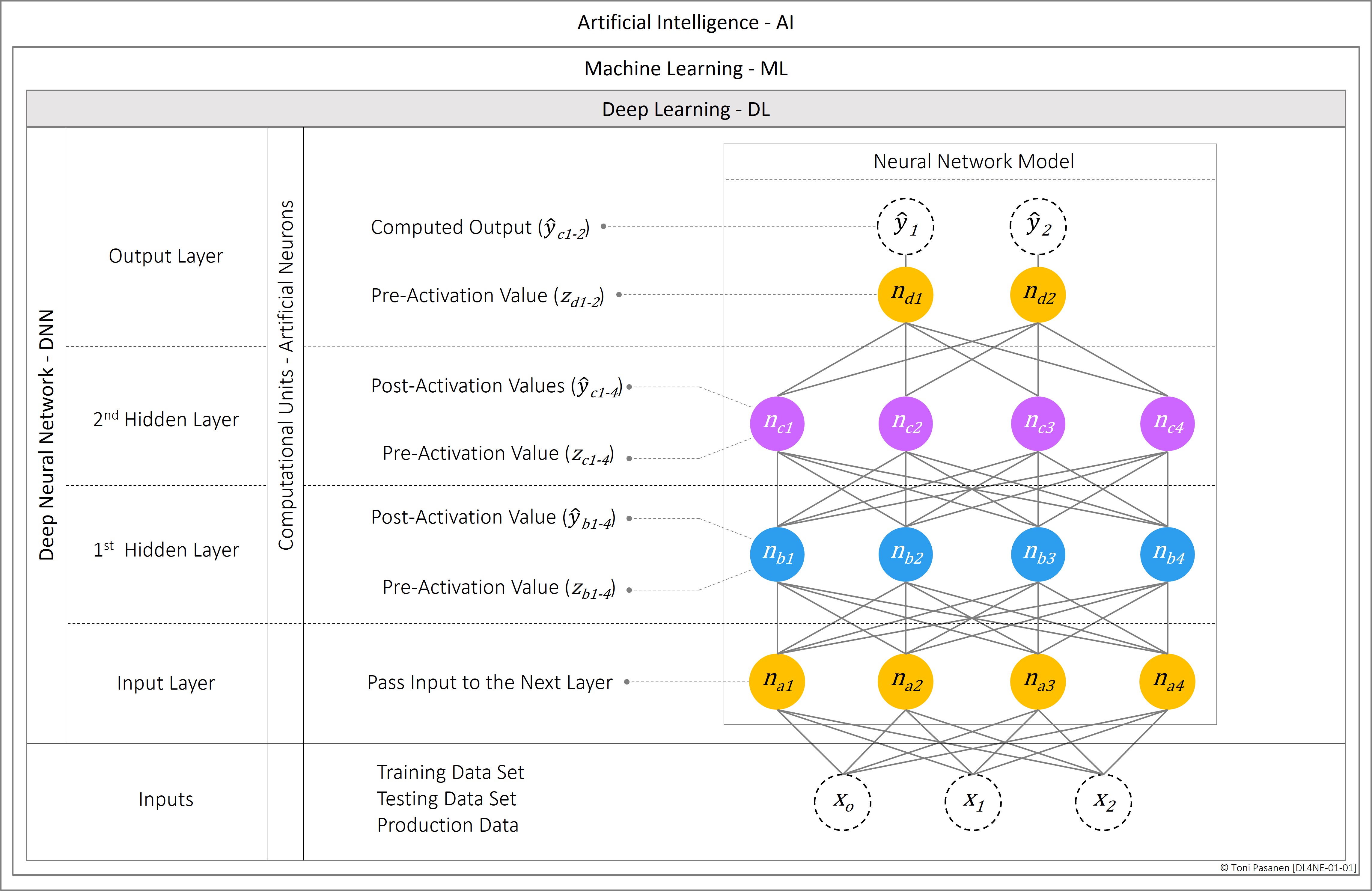
The previous chapter explained how Feed-forward Neural Networks (FNNs) can be used for multi-class classification of 28 x 28 pixel handwritten digits from the MNIST dataset. While FNNs work well for this type of task, they have significant limitations when dealing with larger, high-resolution color images.

In neural network terminology, each RGB value of an image is treated as an input feature. For instance, a high-resolution 600 dpi RGB color image with dimensions 3.937 x 3.937 inches contains approximately 5.58 million pixels, resulting in roughly 17 million RGB values.

If we use a fully connected FNN for training, all these 17 million input values are fed into every neuron in the first hidden layer. Each neuron must compute a weighted sum based on these 17 million inputs. The memory required for storing the weights depends on the numerical precision format used. For example, using the 16-bit floating-point (FP16) format, each weight requires 2 bytes. Thus, the memory requirement per neuron would be approximately 32 MB. If the first hidden layer has 10,000 neurons, the total memory required for storing the weights in this layer would be around 316 GB.

In contrast, Convolutional Neural Networks (CNNs) use shared weight matrices called kernels (or filters) across all neurons within a convolutional layer. For example, if we use a 3x3 kernel, there are only 9 weights per color channel. This reduces memory usage and computational costs significantly during both the forward and backward passes.

Another limitation of FNNs for image recognition is that they treat each pixel as an independent unit. As a result, FNNs do not capture the spatial relationships between pixels, making them unable to recognize the same object if it shifts within the frame. Additionally, FNNs cannot detect edges or other important features. On the other hand, CNNs have a property called translation invariance, which allows the model to recognize patterns even if they are slightly shifted (small translations along the x and y axes). This helps CNNs classify objects more accurately. Furthermore, CNNs are more robust to minor rotations or scale changes, though they may still require data augmentation or specialized network architectures to handle more complex transformations.

 

Convolution Layer

Convolution Process

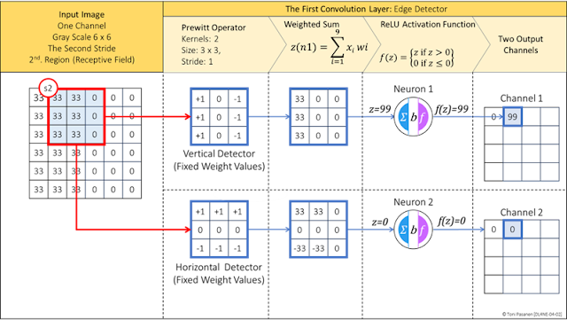
The purpose of the convolution process is to extract features from the image and reduce the number of input parameters before passing them through fully-connected layers. The convolution operation uses a shared weight matrix called kernels or filters, which are shared across all neurons within a convolutional layer. In this example, we use the Prewitt operator, which consists of two 3x3 kernels with fixed weight values for detecting vertical and horizontal edges.

In the first step, these two kernels are positioned over the first region of the input image, and each pixel value is multiplied by the corresponding kernel weight. Next, the process computes the weighted sum, z=0, and the result is passed through the ReLU activation function. The resulting activation values, f(z)=0 , contribute to the neuron-based output channels.

Since our input image is a grayscale image without color channels (unlike an RGB image), it has only one input channel. By using two kernels, we obtain two output channels: one for detecting vertical edges and the other for detecting horizontal edges. The formula for calculating the size of the output channel:

Height = (Image h – Kernel h)/Stride + bias =   (6-3)/1 + 1 = 4

Width = (Image w – Kernel w)/Stride + bias = (6-3)/1 + 1 = 4

Figure 4-1: Convolution Layer – Stride One.

After calculating the first value for the output channel using the image values in the first region, the kernel is shifted one step to the right (stride of 1) to cover the next region. The convolution process calculates the weighted sum based on the values in this region and the weights of the kernel. The result is then passed through the ReLU activation function. The output of the ReLU activation function differs: for the first output channel, it is f(z)=99; for the second output channel, it is f(z)=0. Figure 4-3 depicts the fifth stride.

Figure 4-2: Convolution Layer – Stride Two.

Figure 4-3: Convolution Layer – Stride Five.

The sixteenth stride, shown in Figure 4-4, is the last one. Now output channels one and two are filled.

Figure 4-4: Convolution Layer – Stride Sixteenth.

Figure 4-5 shows how the convolution process found one vertical edge and zero horizontal edge from the input image. The convolution process produces two output channels, each with a size of 4 × 4 pixels, while the original input image was 6 × 6 pixels.

Figure 4-5: Convolution Layer – Detected Edges.

MaxPooling

MaxPooling is used to reduce the size of the output channels if needed. In our example, where the channel size is relatively small (4 × 4), MaxPooling is unnecessary, but we use it here to demonstrate the process. Similar to convolution, MaxPooling uses a kernel and a stride. However, instead of fixed weights associated with the kernel, MaxPooling selects the highest value from each covered region. This means there is no computation involved in creating the new matrix. MaxPooling can be considered as a layer or part of the convolution layer. Due to its non-computational nature, I see it as part of the convolution layer rather than a separate layer.

Figure 4-6: Convolution Layer: MaxPooling.

The First Convolution Layer: Convolution

In this section, we take a slightly different view of convolutional neural networks compared to the preceding sections. In this example, we use the Kirsch operator in the first convolution layer. It uses 8 kernels for detecting vertical, horizontal, and diagonal edges. Similar to the Prewitt operator, the Kirsch operator uses fixed weight values in its kernels. These values are shown in Figure 4-7.

Figure 4-8: Kirsch Operator.

In Figure 4-8, we use a pre-labeled 96 x 96 RGB image for training. An RGB image has three color channels: red, green, and blue for each pixel. It is possible to apply all kernels to each color channel individually, resulting in 3 x 8 = 24 output channels. However, we follow the common practice of applying the kernels to all input channels simultaneously, meaning the eight Kirsch kernels have a depth of 3 (matching the RGB channels). Each kernel processes the RGB values together and produces one output channel. Thus, each neuron uses 3 (width) x 3 (height) x 3 (depth) = 27 weight parameters for calculating the weighted sum. With a stride value of one, the convolution process generates eight 94 x 94 output channels. The formula for calculating weighted sum:

Figure 4-8: The First Convolution Layer – Convolution Process.

The First Convolution Layer: MaxPooling

To reduce the size of the output channels from the first convolution layer, we use MaxPooling. We apply eight 2 x 2 kernels, each with a depth of 8, corresponding to the output channels. All kernels process the channels simultaneously, selecting the highest value among the eight channels. MaxPooling with this setting reduces the size of each output channel by half, resulting in eight 47 x 47 output channels, which are then used as input channels for the second convolution layer

Figure 4-9: The First Convolution Layer – MaxPooling.

The Second Convolution Layer

Figure 4-10 shows both the convolution and MaxPooling processes. The eight 47 x 47 output channels produced by the first convolution layer are used as input channels for the second convolution layer. In this layer, we use 16 kernels whose initial weight values are randomly selected and adjusted during the training process. The kernel size is set to 3 x 3, and the depth is 8, corresponding to the number of input channels. Thus, each kernel calculates a weighted sum over 3 x 3 x 8 = 72 parameters with 72 weight values. All 16 kernels produce new 45 x 45 output channels by applying the ReLU activation function. Before flattening the output channels, our model applies a MaxPooling operation, which selects the highest value within the kernel coverage area (region). This reduces the size of the output channels by half, from 45 x 45 to 22 x 22.

If we had used the original image without convolutional processing as input to the fully connected layer, there would have been 27,648 input parameters (96 x 96 x 3). Thus, the two convolution layers reduce the number of input parameters to 7,744 (22 x 22 x 16), which is approximately a 72% reduction.

Figure 4-10: The Second Convolution Layer – Convolution and MaxPooling.

Fully Connected Layers

Before feeding the data into the fully connected layer, the multi-dimensional 3D array (3D tensor) is converted into a 1D vector. This produces 7,744 input values (22 x 22 x 16) for the input layer. We use 4,000 neurons with the ReLU activation function in the first hidden layer, which is approximately half the number of input values. In the second hidden layer, we have 1,000 neurons with the ReLU function. The last layer, the output layer, has 10 neurons using the SoftMax function. 

Figure 4-11: Fully Connected Layer – Convolution and MaxPooling.

Backpropagation Process

In Fully Connected Neural Networks (FCNNs), every neuron has its own unique set of weights. In contrast, Convolutional Neural Networks (CNNs) use parameter sharing, where the same filter (kernel) is applied across the entire input image. This approach not only reduces the number of parameters but also enhances efficiency.

Additionally, backpropagation in CNNs preserves the spatial structure *) of the input data through convolution and pooling operations. This helps the network learn spatial features like edges, textures, and patterns. In contrast, FCNNs flatten the input data into a 1D vector, losing any spatial information and making it harder to capture meaningful patterns in images.

*) Spatial features refer to the characteristics of an image that describe the relationship between pixels based on their positions. These features capture the spatial structure of the image, such as edges, corners, textures, shapes, and patterns, which are essential for recognizing objects and understanding the visual content.

AI for Network Engineers: Multi-Class Classification

 Introduction 

This chapter explains the multi-class classification training process. It begins with an introduction to the MNIST dataset (Modified National Institute of Standards and Technology dataset). Next, it describes how the SoftMax activation function computes the probability of the image fed into the model during the forward pass and how the weight parameters are adjusted during the backward pass to improve training results. Additionally, the chapter discusses the data parallelization strategy from a network perspective.

MINST Dataset

We will use the MNIST dataset [1], which consists of handwritten digits, to demonstrate the training process. The MNIST dataset includes four files: (1) a training set with 60,000 gray-scale images (28x28 pixels) and their respective (2) labels, and a test set with 10,000 images (28x28 pixels) and their respective labels. Figure 3-1 illustrates the structure and dependencies between the test dataset and the labels.

The file train-images-idx3-ubyte contains metadata describing how the images are ordered, along with the image pixel order. The file train-labels-idx1-ubyte defines which label (the digits 0-9) corresponds to which image in the image file. Since we have ten possible outputs, we use ten output neurons.

Before the training process begins, the labels for each image-label pair are one-hot encoded. This process occurs before the data is fed into the model and involves marking the neuron that corresponds to the digit being represented by the image. For example, image number 142 in Figure 3-1, represents the digit 8, which corresponds to output neuron 9. Note that the first digit, 0, is mapped to neuron 1, so the digit 8 is mapped to neuron 9. One-hot encoding creates a vector of ten values, where the number 1 is placed at the position of the expected neuron, and all other positions are set to 0.

Figure 3-1: Training Dataset & Labels– The MNIST Database.

Forward Pass

Model Probability

Figures 3-2 and 3-3 illustrate the forward pass process for multi-class classification. The input layer flattens the 28x28 pixel image into 784 input parameters, where each parameter represents the intensity of a pixel (0 = black, 255 = white). These 784 input values are then passed to all 128 neurons in the hidden layer. Each neuron in the hidden layer receives all 784 inputs, and each of these inputs is associated with a unique weight. Therefore, each of 128 neurons have 784 weight parameters, and total weight parameter count of hidden layer is 100 352.

In the hidden layer, each neuron computes the weighted sum of its inputs and then applies the ReLU activation function to the result. This process produces 128 activation values—one for each neuron in the hidden layer.

Next, these 128 activation values are fed into the output layer, which consists of 10 neurons (corresponding to the 10 possible classes for the MNIST dataset). Each output neuron is connected to all 128 activation values from the hidden layer. Therefore, the weight parameter counts in the output layer is 1280. Again, each neuron computes the weighted sum of its inputs, and the result of this calculation is called a logit. 

In the output layer, the SoftMax activation function is applied to these logits. SoftMax first computes the exponential of each logit, using Euler’s number e as the base. Then, it computes the sum of these exponentials, which in this example is 24.813. The probability for each class (denoted as y ̂) is calculated by dividing each neuron’s exponential by the sum of all exponentials.

In this example, the output neuron corresponding to class "5" produces the highest probability, meaning the model predicts the digit in the image is 5. However, since this prediction is incorrect in the first iteration, the model will adjust its weights during backpropagation.

In our model, we have 101,632 weight parameters. The number of bits used to store each weight parameter in a neural network depends on the numerical precision chosen for the model. The 32-bit floating point (FP32 – single precision) is the standard precision used, where each weight is represented using 32 bits (4 bytes). This format offers good precision but can be memory-intensive for large models. To reduce memory usage and increase speed, many modern hardware systems use 16-bit floating point (FP16 – half precision), where each weight is represented using 16 bits (2 bytes). There is also 64-bit floating point (FP64 – double precision), which uses 64 bits (8 bytes), providing more precision and a larger range than FP32, but at the cost of increased memory usage.

In our model, using FP32, the memory required for the weight parameters is 406,528 bytes (4 × 101,632).

Figure 3-2: Forward pass – Probability Computation.

Cross-Entropy Loss

In our example, the highest probability value (0.244) is provided by neuron 5, though the expected value should be produced by neuron 9. Next, the algorithm computes the cross-entropy loss by taking the logarithm of the probability value for the expected neuron, as defined by the one-hot encoded label. In our example, the probability of the digit being 8, computed by neuron 9, is 0.181. The cross-entropy loss is calculated by taking the log of 0.181, resulting in 0.734. 

Figure 3-3: Forward pass – Cross-Entropy Loss.

Backward Pass

Gradient Computing

The gradient for the neurons in the output layer is calculated by subtracting the ground truth value (from the one-hot encoding) from the probability generated by the SoftMax function. Although the cross-entropy loss is used during training, it is not directly involved in this gradient calculation. Figure 3-4 illustrates the gradient computation process.

For neurons in the hidden layer, the gradient is computed by multiplying the weighted sum of the gradients from the connected output neurons with the initial weight values. This result is then multiplied by the derivative of the neuron’s own ReLU activation function. The formula is shown in the figure below.

Figure 3-4: Backward pass - Gradient Calculation.

Weight Adjustment Values

After calculating the gradients for all neurons, the backpropagation algorithm determines the weight adjustments. While this process was explained in the previous chapter, let's briefly recap it here. The weight adjustment value is computed by multiplying the gradient of that neuron by the weight-associated input value and the shared hyperparameter, the learning rate. 

Figure 3-5 illustrates the computation from two perspectives: neuron 9 in the output layer and neuron 1 in the hidden layer. 

Figure 3-5: Backward Pass - Weight Adjustment Value.

Weight Update

Figure 3-6 depicts how the new weight value is obtained by adding the adjustment value to the initial weight value. 

Figure 3-6: Backward Pass – Computing New Value for the Weight Parameter.

 

Data Parallelization and Network Impact

So far, we have explored how the backpropagation algorithm functions in multi-class classification on a single GPU. In the next section, we will discuss the process when the input data size exceeds the memory capacity of a single GPU and how we leverage a Data Parallelization Strategy to divide the training data among multiple GPUs. We will also look at the Data Parallelization Strategy from the link utilization perspective.

In Figure 3-7, we have divided the training data into mini-batches. The first half of these mini-batches is stored in system memory DRAM-1 (on Server-1), and the second half is stored in system memory DRAM-2 (on Server-2). This approach demonstrates how, when the data exceeds the memory capacity of a GPU, idle mini-batches can be stored in system memory. The model and its parameters are stored in the GPU’s VRAM alongside the active mini-batch being processed for training.

In our example, each mini-batch composed of 64 images, which the GPU processes in parallel, with each image handled by a dedicated GPU core. Thus, for the first mini-batch, consisting of 64 images, we have 768 neurons (64 x 138), and 6,422,528 weight parameters (128neurons x 64images x 784inputs) + (10neurons x 64images x 128inputs) for the input data, along with 8,832 bias weight parameters. After the forward pass (computation phase), the backward pass begins. During this phase, the backpropagation algorithm calculates the gradients for all neurons.

We employ the All-Reduce collective communication model, where gradients for each layer are summed across mini-batches and synchronized between GPUs. Synchronization happens through direct memory copy using Remote Direct Memory Access (RDMA), enabling GPUs to communicate directly with each other's memory while bypassing the network stack. The RDMA process is covered in detail in a later chapter.

Gradients are summed and synchronized among the GPUs over a network connection. During this synchronization, the GPU’s network interface controller (NIC) forwards packets at line rate, resulting in nearly 100% link utilization. Once synchronization is complete, the GPUs average the gradients and compute new weight adjustment values, which are then used to update all weight parameters. These updated weights are also synchronized between GPUs via RDMA.

Next, the training data is fed back into the model with the newly adjusted weights. During this computation phase, network link utilization is relatively low. The training process typically requires multiple iterations of the forward and backward passes. Once the training results are satisfactory, the adjusted weight values are stored in VRAM, and the processed mini-batch is copied back to system memory, while a new mini-batch is transferred from system memory to the GPU’s VRAM. This transfer usually occurs over the PCIe link, which can introduce delays and increase the overall training time.

To mitigate this, multiple GPUs can be used, allowing the entire training dataset to be stored across their combined memory. This avoids frequent data transfers over PCIe and accelerates the training process. If all GPUs are within the same server, communication occurs over the high-speed NVLink, further enhancing performance.

Due to the time-consuming nature of the training process, which can take several weeks or even months, it is crucial that the communication channel between GPUs is lossless and forwards packets at a line rate. Additionally, regular snapshots of the training results should be taken to guard against potential packet loss, which could occur if the backend network loses even a single packet for any reason. Without these snapshots, the training job would have to start over from the beginning.

Figure 3-7: Gradient Synchronization and Network Utilization.

 

References

1. Yann LeCun, Corina Cortes, Christoper J.C. Burges: The MNIST database of handwritten digits. 

AI for Network Engineers: Backpropagation Algorithm

 Introduction 

This chapter introduces the training model of a neural network based on the Backpropagation algorithm. The goal is to provide a clear and solid understanding of the process without delving deeply into the mathematical formulas, while still explaining the fundamental operations of the involved functions. The chapter also briefly explains why, and in which phases the training job generates traffic to the network, and why lossless packet transport is required. The Backpropagation algorithm is composed of two phases: the Forward pass (computation phase) and the Backward pass (adjustment and communication phase).

In the Forward pass, neurons in the first hidden layer calculate the weighted sum of input parameters received from the input layer, which is then passed to the neuron's activation function. Note that neurons in the input layer are not computational units; they simply pass the input variables to the connected neurons in the first hidden layer. The output from the activation function of a neuron is then used as input for the connected neurons in the next layer. The result of the activation function in the output layer represents the model's prediction, which is compared to the expected value (ground truth) using the error function. The output of the error function indicates the accuracy of the current training iteration. If the result is sufficiently close to the expected value (error function close to zero), the training is complete. Otherwise, it triggers the Backward pass process.

As the first step in the backward pass, the backpropagation algorithm calculates the derivative of the error function, providing the output error (gradient) of the model. Next, the algorithm computes the error term (gradient) for the neuron(s) in the output layer by multiplying the derivative of each neuron’s activation function by the model's error term. Then, the algorithm moves to the preceding layer and calculates the error term (gradient) for its neuron(s). This error term is now calculated using the error term of the connected neuron(s) in the next layer, the derivative of each neuron’s activation function, and the value of the weight parameter associated with the connection to the next layer.

After calculating the error terms, the algorithm determines the weight adjustment values for all neurons simultaneously. This computation is based on the input values, the adjustment values, and a user-defined learning rate. Finally, the backpropagation algorithm refines all weight values by adding the adjustment values to the initial weights. Once the backward pass is complete, the backpropagation algorithm starts a new iteration of the forward pass, gradually improving the model's predictions until they closely match the expected values, at which point the training is complete.

Figure 2-1: Backpropagation Overview.

The First Iteration - Forward Pass

Training a model often requires multiple iterations of forward and backward passes. In the forward pass, neurons in the first hidden layer calculate the weighted sum of input values, each multiplied by its associated weight parameter. These neurons then apply an activation function to the result. Neurons in subsequent layers use the activation output from previous layers as input for their own weighted sum calculations. This process continues through all the layers until reaching the output layer, where the activation function produces the model's prediction.

After the forward pass, the backpropagation algorithm calculates the error by comparing the model's output with the expected value, providing a measure of accuracy. If the model's output is close to the expected value, training is complete. Otherwise, the backpropagation algorithm initiates the backward pass to adjust the weights and reduce the error in subsequent iterations.

 

Neuron-a Forward Pass Calculations

Weighted Sum

In Figure 2-2, we have an imaginary training dataset with three inputs and a bias term. Input values and their respective initial weight values are listed below: 

• x1 = 0.2 , initial weight wa1 = 0.1

• x2 = 0.1, initial weight wa2 = 0.2

• x3 = 0.4 , initial weight wa3 = 0.3

• ba0 = 1.0 , initial weight wa0 = 0.6

From the model training perspective, the input values are constant, unchageable values, while weight values are variables which will be refined during the backward pass process.

The standard way to write the weighted sum formula is: 

Where:

• n = 3 represents the number of input values (x1, x2, x3).

• Each input xi  is multiplied by its respective weight wi, and the sum of these products is added to the bias term b.

In this case, the equation can be explicitly stated as:

Which with our parameters gives:

Activation Function

Neuron-a uses the previously calculated weighted sum as input for the activation function. We are using the ReLU function (Rectified Linear Unit), which is more popular than the hyperbolic tangent and sigmoid functions due to its simplicity and lower computational cost.

The standard way to write the ReLU function is:

Where:

f(a) represents the activation function.

z  is the weighted sum of inputs.

The ReLU function returns the z if z > 0. Otherwise, it returns 0 if z ≤ 0.

In our example, the weighted sum za is 0.76, so the ReLU function returns:

Figure 2-2: Activation Function for Neuron-a.

 

Neuron-b Forward Pass Calculations

Weighted Sum

Besides the bias term value of 1.0,  Neuron-b uses the result provided by the activation function of neuron-a as an input to weighted sum calculation. Input values and their respective initial weight values are listed below: 

This gives us:

Activation Function

Just like Neuron-a, Neuron-b uses the previously calculated weighted sum as input for the activation function. Because the zb = 0.804 is greater than zero, the ReLU activation function f(b) returns:

Neuron-b is in the output layer, so its activation function result y_b represents the prediction of the model. 

 

Figure 2-3: Activation Function for Neuron-b.

Error Function

To keep things simple, we have used only one training example. However, in real-life scenarios, there will always be more than one training example. For instance, a training dataset might contain 10 images of cats and 10 images of dogs, each having 28x28 pixels. Each image represents a training example, giving us a total of 20 training examples. The purpose of the error function is to provide a single error metric for all training examples. In this case, we are using the Mean Squared Error (MSE).

We can calculate the MSE using the formula below where the expected value y is 1.0 and the model’s  prediction for the training example yb = 0.804. This gives an error metric of 0.019, which can be interpreted as an indicator of the model's accuracy.

The result of the error function is not sufficiently close to the desired value, which is why this result triggers the backward pass process.

Figure 2-4: Calculating the Error Function for Training Examples.

 

Backward Pass

In the forward pass, we calculate the model’s accuracy using several functions. First, Neuron-a computes the weighted sum Σ(za ) by multiplying the input values and the bias term with their respective weights. The output, za, is then passed through the activation function f(a), producing ya. Neuron-b, in turn, takes ya and the bias term to calculate the weighted sum Σ(zb ). The activation function f(b) then uses zb to compute the model’s output, yb. Finally, the error function f(e) calculates the model’s accuracy based on the output.

So, dependencies between function can be seen as:

The backpropagation algorithm combines these five functions to create a new error function, enew(x), using function composition and the chain rule. The following expression shows how the error function relates to the weight parameter w1 used by Neuron-a:

This can be expressed using the composition operator (∘) between functions:

Next, we use a method called gradient descent to gradually adjust the initial weight values, refining them to bring the model's output closer to the expected result. To do this, we compute the derivative of the composite function using the chain rule, where we take the derivatives of:

1. The error function (e) with respect to the activation function (b).

2. The activation function b with respect to the weighted sum (zb). 

3. The weighted sum (zb) with respect to the activation function (a).

4. The activation function (a) with respect to weighted sum (za(w1)). 

In Leibniz’s notation, this looks like:

Figure 2-5 illustrates the components of the backpropagation algorithm, along with their relationships and dependencies.

Figure 2-5: The Backward Pass Overview.

Partial Derivative for Error Function – Output Error (Gradient)

As a recap, and for illustrating that the prediction of the first iteration fails, Figure 2-6 includes the computation for the error function (MSE = 0.019). 

As a first step, we calculate the partial derivative of the error function. In this case, the partial derivative describes the rate of change of the error function when the input variable yb changes. The derivative is called partial when one of its input values is held constant (i.e., not adjusted by the algorithm). In our example, the expected value y is constant input. The result of the partial derivative of the error function describes how the predicted output should change yb to minimize the model’s error.

We use the following formula for computing the derivative of the error function:

Figure 2-6: The Backward Pass – Derivative of the Error Function.

The following explanation is meant for readers interested in why there is a minus sign in front of the function.

When calculating the derivative, we use the Power Rule. The Power Rule states that if we have a function f(x) = xn , then its derivative is f’(x) = n ⋅ xn-1. In our case, this applies to the error function:

Using the Power Rule, the derivative becomes:

Next, we apply the chain rule by multiplying this result by the derivative of the inner function (y − yb), with respect to yb . Since y is treated as a constant (because it represents our target value, which doesn't change during optimization), the derivative of (y − yb) with respect to yb  is simply −1, as the derivative of − yb  with respect to yb  is −1, and the derivative of y (a constant) is 0.

Therefore, the final derivative of the error function with respect to yb  is:

Partial Derivative for the Activation Function

After computing the output error, we calculate the derivative of the activation function f(b) with respect to zb . Neuron b uses the ReLU activation function, which states that if the input to the function is greater than 0, the derivative is 1; otherwise, it is 0. In our case, the result of the activation function f(b)=0.804, so the derivative is 1.

Error Term for Neurons (Gradient)

The error term (Gradient) for neuron-b is calculated by multiplying the output error, the partial derivative of the error function,  by the derivative of the neuron's activation function. This means that now we propagate the model's error backward using it as a base value for finetuning the model accuracy (i.e., refining new weight values). This is why the term backward pass fits perfectly for the process.

Figure 2-7: The Backward Pass – Error Term (Gradient) for Neuron-b.

After computing the error term for Neuron-b, the backward pass moves to the preceding layer, the hidden layer, and calculates the error term for Neuron-a. The algorithm computes the derivative for the activation function f(a) = 1, as it did with the Neuron-b. Next, it multiplies the result by Neuron-b's error term (-0.196) and the connected weight parameter , wb1 =0.4. The result -0.0784 is the error term for Neuron-a.

Figure 2-8: The Backward Pass – Error Term (Gradient) for Neuron-a.

Weight Adjustment Value

After computing error terms for all neurons in every layer, the algorithm simultaneously calculates the weight adjustment value for every weight. The process is simple, the error term is multiplied with an input value connected to weight and with learning rate (η). The learning rate balances convergence speed and training stability. We have set it to -0.6 for the first iteration. The learning rate is a hyper-parameter, meaning it is set by the user rather than learned by the model during training. It affects the behavior of the backpropagation algorithm by controlling the size of the weight updates. It is also possible to adjust the learning rate during training—using a higher learning rate at the start to allow faster convergence and lowering it later to avoid overshooting the optimal result. 

 

Weight adjustment value for weight wb1 and wa1 respectively:

Note! It is not recommended to use a negative learning rate. I use it here because we get a good enough output for the second forward pass iteration.

Figure 2-9: The Backward Pass – Weight Adjustment Value for Neurons.

Refine Weights

As the last step, the backpropagation algorithm computes new values for every weight parameter in the model by simply summing the initial weight value and weight adjustment value.

New values for weight  parameters wb1 and wa1 respectively:

Figure 2-10: The Backward Pass – Compute New Weight Values.

The Second Iteration - Forward Pass

After updating all the weight values (wa0, wa1, wa2, and wa3 ), the backpropagation process begins the second iteration of the forward pass. As shown in Figure 2-11, the model output yb = 0.9982 is very close to the expected value y = 1.0. The new MSE = 0.0017, is much better than 0.019 computed in the first iteration.

Figure 2-11: The Second Iteration of the Forward Pass.

Network Impact

Figure 2-12 shows a hypothetical example of Data Parallelization, where our training data set is split into two batches, A and B, which are processed by GPU-A and GPU-B, respectively. The training model is the same on both GPUs: Fully-Connected, with two hidden layers of four neurons each, and one output neuron in the output layer.

After computing a model prediction during the forward pass, the backpropagation algorithm begins the backward pass by calculating the gradient (output error) for the error function. Once computed, the gradients are synchronized between the GPUs. The algorithm then averages the gradients, and the process moves to the preceding layer. Neurons in the preceding layer calculate their gradient by multiplying the weighted sum of their connected neurons’ averaged gradients and connected weight with the local activation function’s partial derivative. These neuron-based gradients are then synchronized over connections. Before the process moves to the preceding layer, gradients are averaged. The backpropagation algorithm executes the same process through all layers. 

If packet loss occurs during the synchronization, it can ruin the entire training process, which would need to be restarted unless snapshots were taken. The cost of losing even a single packet could be enormous, especially if training has been ongoing for several days or weeks. Why is a single packet so important? If the synchronization between the gradients of two parallel neurons fails due to packet loss, the algorithm cannot compute the average, and the neurons in the preceding layer cannot calculate their gradient. Besides, if the connection, whether the synchronization happens over NVLink, InfiniBand, Ethernet (RoCE or RoCEv2), or wireless connection, causes a delay, the completeness of the training slows down. This causes GPU under-utilization which is not efficient from the business perspective.

Figure 2-12: Backward Pass – Gradient Synchronization and Averaging.

To be conntinued...

AI for Network Engineers: Chapter 2 - Backpropagation Algorithm: Introduction

This chapter introduces the training model of a neural network based on the Backpropagation algorithm. The goal is to provide a clear and solid understanding of the process without delving deeply into the mathematical formulas, while still explaining the fundamental operations of the involved functions. The chapter also briefly explains why, and in which phases the training job generates traffic to the network, and why lossless packet transport is required. The Backpropagation algorithm is composed of two phases: the Forward pass (computation phase) and the Backward pass (adjustment and communication phase).

In the Forward pass, neurons in the first hidden layer calculate the weighted sum of input parameters received from the input layer, which is then passed to the neuron's activation function. Note that neurons in the input layer are not computational units; they simply pass the input variables to the connected neurons in the first hidden layer. The output from the activation function of a neuron is then used as input for the connected neurons in the next layer, whether it is another hidden layer or the output layer. The result of the activation function in the output layer represents the model's prediction, which is compared to the expected value (ground truth) using the error function. The output of the error function indicates the accuracy of the current training iteration. If the result is sufficiently close to the expected value, the training is complete. Otherwise, it triggers the Backward pass process.

In the Backward pass process, the Backpropagation algorithm first calculates the derivative of the error function. This derivative is then used to compute the error term for each neuron in the model. Neurons use their calculated error terms to determine how much and in which direction the current weight values must be fine-tuned. Depending on the model and the parallelization strategy, GPUs in multi-GPU clusters synchronize information during the Backpropagation process. This process affects network utilization.

Our feedforward neural network, shown in Figure 2-1, has one hidden layer and one output layer. If we wanted our example to be a deep neural network, we would need to add additional layers, as the definition of "deep" requires two or more hidden layers. For simplicity, the input layer is not shown in the figure.

We have three input parameters connected to neuron-a in the hidden layer as follows:

• Input X1 = 0.2 > neuron-a via weight Wa1 = 0.1

• Input X2 = 0.1 > neuron-a via weight Wa2 = 0.2

• Input X3 = 0.4 > neuron-a via weight Wa3 = 0.3

• Bias ba0 = 1.0 > neuron-a via weight Wa0 = 0.6

The bias term helps ensure that the neuron is active, meaning its output value is not zero.

The input parameters are treated as constant values, while the weight values are variables that will be adjusted during the Backward pass if the training result does not meet expectations. The initial weight values are our best guess for achieving the desired training outcome. The result of the weighted sum calculation is passed to the activation function, which provides the input for neuron-b in the output layer. We use the ReLU (Rectified Linear Unit) activation function in both layers due to its simplicity. There are other activation functions, such as hyperbolic tangent (tanh), sigmoid, and softmax, but those are outside the scope of this chapter.

The input values and weights for neuron-b are:

• Neuron-a activation function output f(af) > neuron-b via weight Wb1

• Bias ba0 = 1.0 > neuron-b via weight Wa0 = 0.5

The output, Ŷ, from neuron-b represents our feedforward neural network's prediction. This value is used along with the expected result, y, as input for the error function. In this example, we use the Mean Squared Error (MSE) error function. As we will see, the result of the first training iteration does not match our expected value, leading us to initiate the Backward pass process.

In the first step of the Backward pass, the Backpropagation algorithm calculates the derivative of the error function (MSE’). Neurons-a and b use this result as input to compute their respective error terms by multiplying MSE’ with the result of the activation function and the weight value associated with the connection to the next neuron. Note that for neuron-b, there is no next layer—just the error function—so the weight parameter is excluded from the error term calculation of neuron-b. Next, the error term value is multiplied by an input value and learning rate, and this adjustment value is added to the current weight.

After completing the Backward pass, the Backpropagation algorithm starts a new iteration of the Forward pass, gradually improving the model's prediction until it closely matches the expected value, at which point the training is complete.

Figure 2-1: Backpropagation Algorithm.

Artificial Intelligence for Network Engineers: Introduction

Several books on artificial intelligence (AI) and deep learning (DL) have been published over the past decade. However, I have yet to find a book that explains deep learning from a networking perspective while providing a solid introduction to DL. My goal is to fill this gap by writing a book titled AI for Network Engineers (note that the title name may change during the writing process). Writing about such a complex subject will take time, but I hope to complete and release it within a year.

Part I: Deep Learning and Deep Neural Networks

The first part of the book covers the theory behind Deep Learning. It begins by explaining the construct of a single artificial neuron and its functionality. Then, it explores various Deep Neural Network models, such as Feedforward Neural Networks (FNN), Convolutional Neural Networks (CNN), and Recurrent Neural Networks (RNN). Next, the first part discusses data and model parallelization strategies such as Data, Pipeline, and Tensor Parallelism, explaining how input data and/or model sizes that exceed the memory capacity of GPUs within a single server can be distributed across multiple GPU servers.

Part II: AI Data Center Networking - Lossless Ethernet

After a brief introduction of RoCEv2, the second part continues from part one by explaining how parallelization strategies affect network utilization. It then discusses the Data Center Quantized Congestion Notification (DCQCN) scheme for RoCEv2, introducing key concepts such as Explicit Congestion Notification (ECN) and Priority-based Flow Control (PFC). In addition to ECN and PFC, this section covers other congestion-avoidance methods, such as packet spraying and deep buffers. The second part also delves into AI data center design choices focusing on the East-West backend network. It introduces Rail, Top-of-Rack (ToR), and Rail-Optimized designs.

Figure 1: Book Introduction.

AI for Network Engineers: Chapter 1 - Deep Learning Basics

Content

Introduction 
Artificial Neuron 
  Weighted Sum for Pre-Activation Value 
  ReLU Activation Function for Post-Activation 
  Bias Term
  S-Shaped Functions – TANH and SIGMOID
Network Impact
Summary
References

Introduction

Artificial Intelligence (AI) is a broad term for solutions that aim to mimic the functions of the human brain. Machine Learning (ML), in turn, is a subset of AI, suitable for tasks like simple pattern recognition and prediction. Deep Learning (DL), the focus of this section, is a subset of ML that leverages algorithms to extract meaningful patterns from data. Unlike ML, DL does not necessarily require human intervention, such as providing structured, labeled datasets (e.g., 1,000 bird images labeled as “bird” and 1,000 cat images labeled as “cat”). 

DL utilizes layered, hierarchical Deep Neural Networks (DNNs), where hidden and output layers consist of computational units, artificial neurons, which individually process input data. The nodes in the input layer pass the input data to the first hidden layer without performing any computations, which is why they are not considered neurons or computational units. Each neuron calculates a pre-activation value (z) based on the input received from the previous layer and then applies an activation function to this value, producing a post-activation output (ŷ) value. There are various DNN models, such as Feed-Forward Neural Networks (FNN), Convolutional Neural Networks (CNN), and Recurrent Neural Networks (RNN), each designed for different use cases. For example, FNNs are suitable for simple, structured tasks like handwritten digit recognition using the MNIST dataset [1], CNNs are effective for larger image recognition tasks such as with the CIFAR-10 dataset [2], and RNNs are commonly used for time-series forecasting, like predicting future sales based on historical sales data. 

To provide accurate predictions based on input data, neural networks are trained using labeled datasets. The MNIST (Modified National Institute of Standards and Technology) dataset [1] contains 60,000 training and 10,000 test images of handwritten digits (grayscale, 28x28 pixels). The CIFAR-10 [2] dataset consists of 60,000 color images (32x32 pixels), with 50,000 training images and 10,000 test images, divided into 10 classes. The CIFAR-100 dataset [3], as the name implies, has 100 image classes, with each class containing 600 images (500 training and 100 test images per class). Once the test results reach the desired level, the neural network can be deployed to production.

Figure 1-1: Deep Learning Introduction.