Introduction
Sequence-to-sequence (seq2seq) language translation and Generative Pretrained Transformer (GPT) models are subcategories of Natural Language Processing (NLP) that utilize the Transformer architecture. Seq2seq models are typically using Long Short-Term Memory (LSTM) networks or encoder-decored based Transformers. In contrast, GPT is an autoregressive language model that uses decoder-only Transformer mechanism. The purpose of this chapter is to provide an overview of the decoder-only Transformer architecture.
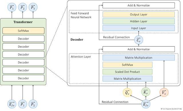
The Transformer consists of stacks of decoder modules. A word embedding vector, a result of the word tokenization and embbeding, is fed as input to the first decoder module. After processing, the resulting context vector is passed to the next decodeer, and so on. After the final decoder, a softmax layer evaluates the output against the complete vocabulary to predict the next word. As an autoregressive model, the predicted word vector from the softmax layer is converted into a token before being fed back into the subsequent decoder layer. This process involves a token-to-word vector transformation prior to re-entering the decoder.
Each decoder module consists of an attention layer, Add & Normalization layer and a feedforward neural network (FFNN). Rather than feeding the embedded word vector (i.e., token embedding plus positional encoding) directly into the decoder layers, the Transformer first computes the Query (Q), Key (K), and Value (V) vectors from the word vector. These vectors are then used in the self-attention mechanism. Initially, the query vector is multiplied by the key vectors using matrix multiplication. The result is then divided by the square root of the dimension of the key vectors (scaled dot product) to obtain the logits. The logits are processed by a softmax layer to compute probabilities. The SoftMax prediction results are multiplied with the value vectors to produce a context vector.
Before feeding the context vector into the feedforward neural network, it is summed with the original word embedding vector (which includes positional encoding) via a residual connection. Finally, the output is normalized using layer normalization. This normalized output is then passed as input to the FFNN, which computes the output.
The basic architecture of the FFNN in the decoder is designed so that the input layer has as many neurons as the dimension of the context vector. The hidden layer, in turn, has four times as many neurons as the input layer, while the output layer has the same number of neurons as the input layer. This design guarantees that the output vector of the FFNN has the same dimension as the context vector. Like the attention block, the FFNN block also employs residual connections and normalization.
Figure 7-8: Decoder-Only Transformer Architecture.
Query, Key and Value Vectors
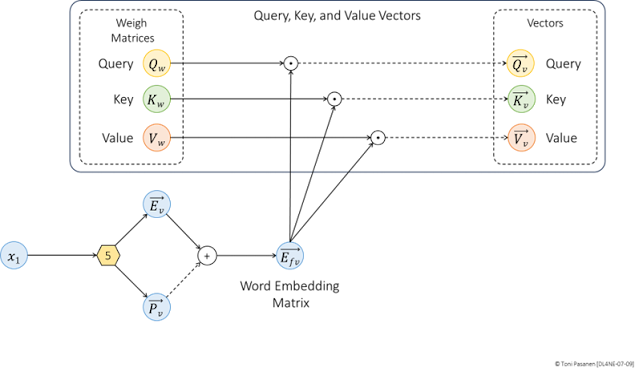
As pointed out in the Introduction, the word embedding vector is not used as input to the first decoder. Instead, it is multiplied by pretrained Query, Key, and Value weight matrices. The result of this matrix multiplication, dot product, produces the Query, Key, and Value vectors, which are use as inputs, and are processed through the Transformer. Figure 7–9 show the basic workflow of this process.
Figure 7-9: Query, Key, and Value Vectors.
Let’s take a closer look at the process using numbers. After tokenizing the input words and applying positional encoding, we obtain a final 5-dimensional word matrix. To reduce computation cycles, the process reduces the dimension of the Query vector from 5 to 3. Because we want the Query vector to be three-dimensional, we use three 5-dimensional column vectors, each of which is multiplied by the word vector.
Figure 7-10: Calculating the Query Vector.
Figure 7–11 depicts the calculation process, where each component of the word vector is multiplied by its corresponding component in the Query weight matrix. The weighted sum of these results forms a three-dimensional Query vector. The Key and Value vectors are calculated using the same method.
The same Query, Key, and Value (Q, K, V) weight matrices are used across all words (tokens) within a single self-attention layer in a Transformer model. This ensures that each token is processed in the same way, maintaining consistency in the attention computations. However, each decoder layer in the Transformer has its own dedicated Q, K, and V weight matrices, meaning that every layer learns different transformations of the input tokens, allowing deeper layers to capture more abstract representations.
Figure 7-11: Calculating the Query Vector.
Attention Layer
Figure 7-12 depicts what happens in the first three components of the Attention layer after calculating the Query, Key, and Value vectors. In this example, we focus on the word “clear”, and try to predict the next word. Its Query vector is multiplied by its own Key vector as well as by all the Key vectors generated for the preceding words. Each multiplication produces its own score. Note that the score values shown in the figure are theoretical and are not derived from the actual Qv × Kv matrix multiplication; however, the remaining values are based on these calculations. Additionally, in our example, we use one-dimensional values (instead of actual vectors) to keep the figures and calculations simple. In reality, these are n-dimensional vectors.
After the Qv × Kv matrix multiplication, the resulting scores are divided by the square root of the vector depth, yielding logits, i.e., the input values for the softmax function. The softmax function then computes the exponential of each logit (using Euler’s number, approximately 2.71828) and divides each result by the sum of all exponentials. For example, the value 3.16, corresponding to the first word, is divided by 482.22, resulting in a probability of 0.007. Note that the sum of the probabilities is 1.0. Softmax ensures that the attention scores sum to 1, making them interpretable as probabilities and helping the model decide which input tokens to focus on when generating an output. In our example, the token for the word “clear” has the highest probability at this stage. The word “decided” has the second highest probability score (0.210), which indicates that the semantics of “clear”, which has the highest probability score (0.665), can be interpreted as an verb answering the question: “What she decided to do?
Figure 7-12: Attention Layer, the First Three Steps.
Next, the SoftMax probabilities are multiplied by each token's Value vector (matrix multiplication). The resulting vectors are then summed, producing the Context vector for the token associated with the word “clear.” Note that the components of the Value vectors are example values and are not derived from actual computations.
Figure 7-13: Attention Layer, the Fourth Step.
Add & Normalization
As the final step, the Word vector, which includes positional encoding, is added to the context vector via a Residual Connection. The result is then passed through a normalization process, where the vector’s components are summed and divided by the vector’s dimension, yielding the mean (μ). This mean value is then used for standard deviation calculation: the mean is subtracted from each of the three vector components, and the results are squared. These squared values are then summed, divided by three (the vector’s dimension), and the square root of this result gives the final output vector [1.40, -0.55, -0.87] of the Add & Normalize layer.
Figure 7-14: Add & Normalize Layer – Residual Connection and Layer Normalization.
Feed Forward Neural Network
Within the decoder module, the feedforward neural network uses the output vector from the Add & Normalize layer as its input. In our example, the FFNN have one neuron in input layer for each component of the vector. This layer simply passes the input values to the hidden layer, where each neuron first calculates a weighted sum and then applies the ReLU activation function. In our example, the hidden layer contains nine neurons (three times the number of input neurons). The output from the hidden layer is then fed to the output layer, where the neurons again compute a weighted sum and apply the ReLU activation function. Note that in transformer-based decoders, the FFNN is applied to each token individually. This means that each token-related output from the attention layer is processed separately by the same FFNN model with shared weights, ensuring a consistent transformation of each token's representation regardless of its position in the sequence.

Figure 7-15: Fully Connected Feed Forward Neural Network (FFNN).
The final decoder output is computed in the Add & Normalize layer, similarly as Add & Normalize after the attention layer. This produces the decoder output, which is used as the input for the next decoder module.
Figure 7-16: Add & Normalize Layer – Residual Connection and Layer Normalization.
Next Word Probability Computation – SoftMax Function
The output of the last decoder module does not directly represent the next word. Instead, it must be transformed into a probability distribution over the entire vocabulary. First, the decoder output is passed through a weight matrix that maps it to a new vector, where each element corresponds to a word in the vocabulary. For example, in Figure 7-17 the vocabulary consists of 12 words. These words are tokenized and linked to their corresponding word embeddings vector. That said, the word embedding matrix serves as a weight matrix.
Figure 7-17: Hidden State Vector and Word Embedding Matrix.
Figure 7-18 illustrates how the decoder output vector (i.e., the hidden state h) is multiplied by all word embedding vectors to produce a new vector of logits.
Figure 7-18: Logits Calculation – Dot Product of Hidden State and Complete Vocabulary.
Next, the SoftMax function is applied to the logits. This function converts the logits into probabilities by exponentiating each logit and then normalizing by the sum of all exponentiated logits. The result is a probability distribution in which each value represents the likelihood of selecting a particular word as the next token.
Figure 7-19: Probability Calculation - Adding Logits to SoftMax Function
Finally, the word with the highest probability is selected as the next token. This token is then mapped back to its corresponding word using a token-to-word lookup. This initiates the next iteration, where the token is converted into its word embedding vector, and used together with positional encoding to create the actual word embedding for the next iteration.
Figure 7-20: Word-to-Token, and Token-to-Word Embedding Process.
In theory, our simple example shows that the model can assign the highest probability to the correct word. For instance, by analyzing the position of the word “clear” relative to its preceding words, the model is able to infer the context. When the context implies that an action is directed toward a known target, the article “the” receives the highest probability score and is predicted as the next word.
Conclusion
We use pretty simple examples in this chapter. However, GPT-3, for example, is built on a deep Transformer architecture comprising 96 decoder blocks. Each decoder block is divided into three primary sub-layers:
Attention Layer: This layer implements multi-head self-attention using four key weight matrices, one each for the query, key, and value projections, plus one for the output projection. Together, these matrices account for roughly 600 million trainable parameters per block.
Add & Normalize Layers: Each block employs two residual connections paired with layer normalization. The first Add & Normalize operation occurs immediately after the Attention Layer, and the second follows the Feed-Forward Neural Network (FFNN) layer. Although essential for stabilizing training, the parameters in each normalization step are relatively few, typically on the order of tens of thousands.
Feed-Forward Neural Network (FFNN) Layer: The FFNN consists of two linear transformations with an intermediate expansion (usually about four times the model’s hidden size). This layer contributes approximately 1.2 billion parameters per block.
Aggregating the parameters from all 96 decoder blocks, and including additional parameters from the token embeddings, positional encodings, and other components, the entire GPT-3 model totals around 175 billion trainable parameters. This is why parallelism is essential: the training process must be distributed across multiple GPUs and executed according to a selected parallelization strategy. The second part of the book discusses about Parallelization.


No comments:
Post a Comment