Model Parallelism with Pipeline Parallelism

 

In Model Parallelism, the neural network is partitioned across multiple GPUs, with each GPU responsible for specific layers of the model. This strategy is particularly beneficial for large-scale models that surpass the memory limitations of a single GPU.

Conversely, Pipeline Parallelism involves dividing the model into consecutive stages, assigning each stage to a different GPU. This setup allows data to be processed in a pipeline fashion, akin to an assembly line, enabling simultaneous processing of multiple training samples. Without pipeline parallelism, each GPU would process its inputs sequentially from the complete dataset, while all other GPUs remain idle.

Our example neural network in Figure 8-3 consists of three hidden layers and an output layer. The first hidden layer is assigned to GPU A1, while the second and third hidden layers are assigned to GPU A2 and GPU B1, respectively. The output layer is placed on GPU B2. The training dataset is divided into four micro-batches and stored on the GPUs. These micro-batches are fed sequentially into the first hidden layer on GPU A1. 

Note 8-1. In this example, we use a small training dataset. However, if the dataset is too large to fit on a single GPU, we combine model parallelism, pipeline parallelism, and data parallelism to distribute the workload efficiently. See the note 8-2 for more detail.

I have divided the forward pass and backward pass into time steps, which are further split into computation and communication phases.

During the forward pass, neurons first calculate the weighted sum of inputs, apply the activation function, and produce an output y (computation phase). The computed outputs y, stored in GPU memory, are then transferred to peer GPU(s) using Remote Direct Memory Access (RDMA) (communication phase).

During the backward pass, the backpropagation algorithm computes the model error (computation phase) and propagates it backward across GPUs using RDMA (communication phase). This process was explained in detail in Chapter 2. 

Note 8-2: In our example, Hidden Layer 1 fits entirely on GPU A1. The same applies to other layers—they each fit within a single GPU. However, if the input dataset is too large to fit into a single GPU, it must be split across multiple GPUs. In that case, Hidden Layer 1 will be distributed across multiple GPUs, with each GPU handling a different portion of the dataset. When this happens, the gradients of Hidden Layer 1 must be synchronized across all GPUs that store part of the layer.

Time step 1:

     Computing:

·    A1 processes the input x1 resulting the output y1.

Communication:

·    A1 transports y1 to A2. 

Active GPUs (25%): A1

Figure 8-3: Model Parallelism with Pipeline Parallelism – Time Step 1.

 

Time step 2: 

Computing:

·    A1 processes the input x2 and produces the output y2.

·    A2 processes the input y1 and produces the output y1.

Communication:

·    A1 transports y2 to A2.

·    A2 transports y1 to B3. 

Active GPUs (50%): A1, A2

Figure 8-4: Model Parallelism with Pipeline Parallelism – Time Step 2.

 

Time step 3:

Computing:

·    A1 processes the input x3 and produces the output y3.

·    A2 processes the input y2 and produces the output y2.

·    B1 processes the input y1 and produces the output y1.

Communication:

·    A1 transports y3 to A2.

·    A2 transports y2 to B1.

·    B1 transports y1 to B2

 Active GPUs (75%): A1, A2, B1

 

Figure 8-5: Model Parallelism with Pipeline Parallelism – Time Step 3. 

Time step 4: 

Computing:

·    A1 processes the input x4 and produces the output y4.

·    A2 processes the input y3 and produces the output y3.

·    B1 processes the input y2 and produces the output y2.

·    B2 processes the input y1 and produces the model output 1.

Communication:

·    A1 transports y3 to A2.

·    A2 transports y2 to B1.

·    B1 transports y1 to B2 

Active GPUs (100%): A1, A2, B1, B2

Figure 8-6: Model Parallelism with Pipeline Parallelism – Time Step 4. 

Time step 5:

Computing:

·    A2 processes the input y4 and produces the output y4.

·    B1 processes the input y3 and produces the output y3.

·    B2 processes the input y2 and produces the model output 2.

·    B2 Computes local neuron error E1, and gradient G1.

Communication:

·    A2 transports y4 to B1.

·    B1 transports y3 to B2.

·    B2 transports error E1 to B1

Active GPUs (75%): A2, B1, B2

 The notation x3 above G1 on GPU B2 indicates that the algorithm computes gradients from the error for each weight associated with the inputs, including the bias. This process is repeated with all four micro-batches. This notation will be used in the upcoming figures as well.

Figure 8-7: Model Parallelism with Pipeline Parallelism – Time Step 5. 

Time step 6: 

Computing:

·    B1 processes the input y4 and produces the output y4.

·    B2 processes the input y3 and produces model output 3.

·    B2 Computes local neuron error E2, and gradient G2.

·    B1 Computes local neuron error E1, and gradient G1.

Communication:

·    B1 transports y4 to B2.

·    B2 transports error E2 to B1

 Active GPUs (50%): B1, B2

 

 Figure 8-8: Model Parallelism with Pipeline Parallelism – Time Step 6. 

Time step 7: 

Computing:

·    B2 processes the input y4 and produces model output 4.

·    B2 Computes local neuron error E3, and gradient G3.

·    B1 Computes local neuron error E2, and gradient G2.

·    A2 Computes local neuron error E1, and gradient G1.

Communication:

·    B2 transports error E3 to B1

·    B1 transports error E2 to A2

·    A2 transports error E1 to A1 

Active GPUs (75%): A2, B1, B2

 

 

Figure 8-9: Model Parallelism with Pipeline Parallelism – Time Step 7. 

Time step 8: 

Computing: 

·    B2 Computes local neuron error E4, and gradient G4.

·    B1 Computes local neuron error E3, and gradient G3.

·    A2 Computes local neuron error E2, and gradient G2.

·    A1 Computes local neuron error E1, and gradient G1.

Communication:

·    B2 transports error E4 to B1

·    B1 transports error E3 to A2

·    A2 transports error E2 to A1 

Active GPUs (100%): A1, A2, B1, B2

 

Figure 8-10: Model Parallelism with Pipeline Parallelism – Time Step 8. 

Time step 9: 

Computing: 

·    B1 Computes local neuron error E4, and gradient G4.

·    A2 Computes local neuron error E3, and gradient G3.

·    A1 Computes local neuron error E2, and gradient G2.

Communication: 

·    B1 transports error E4 to A2

·    A2 transports error E3 to A1 

Active GPUs (75%): A1, A2, B1

 

Figure 8-11: Model Parallelism with Pipeline Parallelism – Time Step 9. 

Time step 10:

Computing: 

·    A2 Computes local neuron error E4, and gradient G4.

·    A1 Computes local neuron error E3, and gradient G3.

Communication: 

·    A2 transports error E4 to A1 

Active GPUs (50%): A1, A2

 

Figure 8-12: Model Parallelism with Pipeline Parallelism – Time Step 10. 

Time step 11: 

Computing: 

·    A1 Computes local neuron error E4, and gradient G4.

Communication: 

Active GPUs (25%): A1

 

In our example, the micro-batches fit into a single GPU, so we don’t need to split them across multiple GPUs. That said, once GPU A1 has computed the gradients for the last micro-batch, the weights are adjusted, and the second iteration of the forward pass begins.

 

Figure 8-13: Model Parallelism with Pipeline Parallelism – Time Step 11. 

If the test dataset is too large for a single GPU and must be split across multiple GPUs, the layers must also be shared between GPUs. For example, hidden layer 1 is on GPUs A1 and C1, while hidden layer 2 is on GPUs A2 and C2. This requires intra-layer gradient synchronization between GPUs sharing the same layer, resulting in inter-GPU packet transport. Figure 8-14 illustrates how gradients are first synchronized (inter-layer). Then, each GPU averages the gradients (sum of gradients divided by the number of GPUs). Finally, the averaged gradients are synchronized.

 

Figure 8-14: Model Parallelism with Pipeline Parallelism – Synchronization.

Parallelism Strategies in Deep Learning

Introduction

Figure 8-1 depicts some of the model parameters that need to be stored in GPU memory: a) Weight matrices associated with connections to the preceding layer, b) Weighted sum (z), c) Activation values (y), d) Errors (E), e) Local gradients (local ∇), f) Gradients received from peer GPUs (remote ∇), g) Learning rates (LR), and h) Weight adjustment values (Δw).

In addition, the training and test datasets, along with the model code, must also be stored in GPU memory. However, a single GPU may not have enough memory to accommodate all these elements. To address this limitation, an appropriate parallelization strategy must be chosen to efficiently distribute computations across multiple GPUs.

This chapter introduces the most common strategies include data parallelism, model parallelism, pipeline parallelism, and tensor parallelism.

Figure 8-1: Overview of Neural Networks Parameters.

Data Parallelism

In data parallelization, each GPU has an identical copy of the complete model but processes different mini-batches of data. Gradients from all GPUs are averaged and synchronized before updating the model. This approach is effective when the model fits within a single GPU’s memory.

In Figure 8-2, the batch of training data is split into eight micro-batches. The first four micro-batches are processed by GPU A1, while the remaining four micro-batches are processed by GPU A2. Both GPUs share the same model, and their input data are processed through all layers to generate a model prediction. The computation during the forward pass does not involve network load traffic. After computing the model error, the backpropagation algorithm starts the backward pass. The first step involves calculating the derivative of the model error, which is synchronized across the GPUs. Next, the error is propagated backward to calculate neuron-based errors, which are then used to compute gradients for each weight parameter. These gradients are synchronized across the GPUs.

The backpropagation algorithm running on GPUs then sums the gradients and divides the result by the number of GPUs. This averaged result is also synchronized across GPUs. In this way, during the backward pass, both local gradients and averaged gradients are synchronized.

In our simple two-GPU example, this process does not generate excessive network traffic, although the GPUs can use 100% of their NICs (network interface cards) forwarding capacity. However, if hundreds or even thousands of GPUs are used, the network traffic becomes significantly larger.

Inter-GPU network communication within a single server (using PCIe, NVLink) or between multiple servers (over InfiniBand, Ethernet, wireless) requires packet forwarding with minimal latency and in a lossless manner. Minimal latency is required to keep the training time as short as possible, while lossless transport is essential because training will pause if even a single packet is lost during synchronization. In the worst-case scenario, if no snapshot of the training progress is taken, the entire training process must be restarted from the beginning. Training a Large Language Model can take months or more.

Now, consider the electricity costs if training had already been running for two months and had to be restarted due to a single packet loss.

Power Consumption Example:

• A single GPU consumes roughly 350W under full load.
• Total power consumption for 50,000 GPUs: 350 W×50,000=17,500,000 W=17.5 MW
• For two months (60 days = 1,440 hours) of training: 17.5 MW×1,440 hours=25,200 MWh=25,200,000
• If electricity costs $0.10 per kWh, the total training cost will be: 25,200,000 kWh×0.10=2,520,000 USD

Figure 8-2: Data Parallelism Overview.

Training Neural Networks: Backpropagation Algorithm

 Introduction 

The previous chapter explained the operation of a single artificial neuron. It covered how input values are multiplied by their respective weight parameters, summed together, and combined with a bias term. The resulting value, z, is then passed through a non-linear sigmoid function, which squeezed a neuron’s output value y ̂ between 0 and 1.

In this chapter, we form the smallest possible Feed Forward Neural Network (FFNN) model using only two neurons. While this is far from a Deep Neural Network (DNN), a simple NN with two neurons is sufficient to explain the Backpropagation algorithm, which is the focus of this chapter.

The goal is to demonstrate the training process and illustrate how the Forward Pass (computation phase) first generates a model output, y ̂. The algorithm then evaluates the model’s accuracy by computing the error term using Mean Squared Error (MSE). The first training iteration rarely, if ever, produces a perfect output. To gradually bring the training result closer to the expected value, the Backward Pass (adjustment and communication phase) calculates the magnitude and direction by which the weight values should be adjusted. The Backward Pass is repeated as many times as necessary until an acceptable model output is achieved. We are using a supervised training process with a pre-labeled test dataset, although it is not shown in Figure 2-1. Chapter Three covers the training datasets in detail.

After the training process is completed, we use a test dataset to evaluate the model's performance. Test dataset also contains input data and labels, but these labels are not used during training. Instead, after training is complete, the model is evaluated on the test dataset to measure its performance. At this phase, we measure how well the predictions from the training and test phases align. When the model produces the expected results on the test dataset, it can be taken into production.

 

Forward Pass

Figure 1-1 illustrates how neuron-a computes a weighted sum from three input values, adds a bias term, and produces a pre-activation value za. This value is then passed through the Sigmoid activation function. The output y ̂a from neuron-a serves as an input for neuron-b, which processes it and generates the final model output y ̂b. Since these computational steps were covered in detail in Chapter 1, we will not repeat them here.

As the final step of the Forward Pass, we apply the error function E to the model output. The error function measures how far model output y ̂b is from expected value y. We use the Mean Squared Error (MSE), which is computed by subtracting the expected value from the model’s output, squaring the result, and multiplying it by 0.5 (or equivalently, dividing by two).

Figure 2-1: An Overview of a Complete Forward Pass Process.

On the right side of Figure 2-2, we have a two-dimensional error space. In this space, a symmetric parabolic curve visualizes the error function. The curve is centered at the expected value, which is 1.0 in our example. The horizontal axis represents the model output, y, and the vertical axis represents the error. For instance, if the model prediction is 1.7, you can draw a vertical line from this point on the horizontal axis to meet the parabolic curve. In our case, this intersection shows an error term of 0.245. In real-life scenarios, the error landscape often has many peaks and valleys rather than a simple symmetric curve.

The Mean Squared Error (MSE) is a loss function that measures the difference between the predicted values and the expected values. It provides an overall error value for the model, which is also called the loss or cost, indicates how far off the predictions are.

Next, the gradient is computed by taking the derivative of the loss function with respect to the model's weights. This gradient shows both the direction and the magnitude of the steepest increase in error. During the Backward Pass, the algorithm calculates the gradient for each weight. By moving in the opposite direction of the gradient (using a method called Gradient Descent), the algorithm adjusts the weights to reduce the loss. This process is repeated many times so that the model output gradually becomes closer to the expected value. 

The following sections will cover the processes and computations performed during the Backward Pass.

Figure 2-2: Mean Square Error.

 

Learning Rate

Besides determining the direction in which the error should be reduced, the process also needs to know the size of each adjustment step. This is defined by the Learning Rate. The Learning Rate value affects  how much the weights are adjusted in response to the gradient during each iteration of the Backward Pass. A small Learning Rate leads to small, gradual changes, which may result in slower training but a more stable convergence. On the other hand, a large Learning Rate can speed up training by making larger adjustments, yet it might overshoot the optimal values and cause instability. Therefore, choosing the right Learning Rate is crucial for effective and efficient training. This is illustrated in the Figure 2-3. We will get back to Learning Rate in the Backward Pass section.

Figure 2-3: Learning Rate.

 

Backward Pass

The Forward Pass produces the model output ŷ, which is then used to compute the model error E. The closer ŷ is to the expected value y, the smaller the error, indicating better model performance. The purpose of the Backward Pass, as part of the Backpropagation algorithm, is to adjust the model’s weight parameters during training in a direction that gradually moves the model’s predictions closer to the expected values y.

In Figure 2-4, the model’s output ŷb depends on the weighted sum zb of neuron-b. This weighted sum zb, in turn, is calculated by multiplying an input value ya by its associated weights w1. The same process applies to neuron-a. Backpropagation algorithm cannot directly modify the results of an activation function or the weighted sum itself. Nor can it alter the input values directly. Instead, it calculates weight adjustments, which are then used to update the model’s weights.

Figure 2-4 illustrates this dependency chain and provides a high-level overview of how the Backpropagation algorithm determines weight adjustments. The following sections will explain this process in detail.

Figure 2-4: Backpropagation Overview: Backward Pass Dependency Chain.

The somewhat crowded Figure 2-5 illustrates the components of the backpropagation algorithm, along with their relationships and dependencies. The figure consists of three main blocks. The rightmost block depicts the calculation of the error function. The middle and left blocks outline the steps for defining and adjusting new weight values. The complete backward pass process is explained next in detail, one step at a time.

Figure 2-5: The Backward Pass Overview.

Partial Derivative for Error Function – Output Error (Gradient)

The goal of training a model is to minimize the error, meaning we want yb  (the model's prediction/output) to get as close as possible to y (the expected value). 

After computing the error E = 0.245, we compute the partial derivative of the error function with respect to yb  = 1.7, which shows how small changes in yb affect the error E.  A derivative is called partial when one of its input values is held constant (i.e., not adjusted by the algorithm). In our example, the expected value y is constant input. The result of the partial derivative of the error function indicates how the predicted output yb  should change to minimize the model’s error.

We use the following formula for computing the derivative of the error function:

MSE'=- (y-yb)

MSE'=- (1.0-1.7)

MSE'=0.7

Since the model output yb =1.7 is too high, the positive gradient suggests that it should be lowered by 0.7, which is the derivative of the error function (MSE’). This makes perfect sense because by subtracting the MSE's 0.7 from the model output yb = 1.7, we obtain 1.0, which matches the expected value.

Figure 2-6: The Backward Pass – Derivative of the Error Function.

 

Partial Derivative for the Activation Function

After computing the output error, we calculate the derivative of the activation function f(b) with respect to zb . Neuron-b uses a ReLU activation function, which states that if the function’s output is greater than 0, the derivative is 1; otherwise, it is 0. In our case, the result of the activation function f(b)=1.7, so the derivative is 1.

Error Term for Neurons

The error term for neuron-b is calculated by multiplying the partial derivative of the error function MSE’ = 0.7,  by the derivative of the neuron's activation function f^' (b)= 1.0. This means we propagate the model's error backward using it as a base value for finetuning the model accuracy (i.e., refining new weight values). This is why the term backward pass fits perfectly for the process.

Error term (Enb) for Neuron-b = MSE’ ⋅f^' (b)= 0.7 ⋅1=0.7

Figure 2-7: The Backward Pass – Error Term for Neuron-b.

After computing the error term for neuron-b, the backward pass moves to the preceding layer, the hidden layer, to calculate the error term for neuron a. First, the process computes a weighted sum of w ⋅ E across all connected neurons in the next layer, output layer in our example. This sum is then multiplied by the derivative of the activation function, f'(a). Since neuron-a is only connected to neuron-b, its error term is calculated as w1⋅ Enb ⋅ f'(a), resulting error term for neuron-a, Ean = 0.4 ⋅ 0.7 ⋅ 1= 0.28.

Figure 2-8: The Backward Pass – Error Term for Neuron-a.

 

Weight Adjustment Value

Gradient Calculation

After computing the error terms for all neurons in every layer, the algorithm simultaneously calculates weight-based gradients. Each gradient is determined by multiplying the input value by the corresponding error term.

In our example, the gradient for weight wa1 , which connects input x1 to neuron-a, is calculated by multiplying the input value x1 (=3.0) by the error term Enb of neuron-a (=0.28), resulting in a gradient of 0.84. Similarly, the gradient for weight wb1 in neuron-b is computed by multiplying the output y (=3.0) of the activation function from neuron-a by the error term Enb  of neuron b (=0.7), yielding a gradient of 2.1.

If the test dataset is divided across multiple GPUs, gradients must be synchronized before computing the actual weight-based adjustment values. Each GPU sums all received gradients, including its own. The sum is then averaged by dividing it by the number of GPUs.

Next, the GPUs synchronize these averaged gradients to ensure that each one uses the same values when calculating the final weight adjustments. This process is part of a data parallelization strategy, where the training dataset is too large to fit into a single GPU’s memory and is split into micro-batches. Each GPU processes its micro-batches using the same model with the same parameters.

Figure 2-9: The Backward Pass – Gradient for Neurons.

 

Weight Adjustment

The weight adjustment value is computed by multiplying the gradient, averaged in our example, by the learning rate η. We use a learning rate of 0.012. This results in a weight adjustment of 0.042 for weight wa1 and 0.105 for weight wb1.

The weight adjustment values are then subtracted from the initial weights. This yields an updated weight of 0.058 (0.1−0.042) for wa1 and 0.295 (0.4−0.105) for wb1.

Figure 2-10: The Backward Pass – Compute New Weight Values.

 

The Second Iteration - Forward Pass

After updating all the weight values, including those associated with biases, the backpropagation process begins the second iteration of the forward pass. As shown in Figure 2-11, the model output y ̂b = 1.28 is very close to the expected value y = 1.0. The new MSE = 0.007 is significantly lower than the initial MSE = 0.245 computed in the first iteration.

Figure 2-11: The Second Iteration of the Forward Pass.

In Figure 2-12, we have two 2-dimensional error spaces. Using the initial weight values, the model output is 1.7, resulting in an MSE of 0.245. After adjusting the weights, the model prediction is 1.119, reducing the MSE to 0.007.

Figure 2-12: Results Comparison.

Network Impact

In figure 2-13 we have a fully-connected Feed Forward Neural Network (FFNN) with four layers; input layer, two hidden layers, and output layer. Training data set is split into two batches, A and B, which are processed by GPU-A and GPU-B. 

After computing a model prediction during the forward pass, the backpropagation algorithm begins the backward pass by calculating the gradient (output error) for the error function. Once computed, the gradients are synchronized between the GPUs. The algorithm then averages the gradients, and the process moves to the preceding layer. Neurons in the preceding layer calculate their gradient by multiplying the weighted sum of their connected neurons’ averaged gradients and connected weight with the local activation function’s partial derivative. These neuron-based gradients are then synchronized over connections. Before the process moves to the preceding layer, gradients are averaged. The backpropagation algorithm executes the same process through all layers. 

If packet loss occurs during the synchronization, it can ruin the entire training process, which would need to be restarted unless snapshots were taken. The cost of losing even a single packet could be enormous, especially if training has been ongoing for several days or weeks. Why is a single packet so important? If the synchronization between the gradients of two parallel neurons fails due to packet loss, the algorithm cannot compute the average, and the neurons in the preceding layer cannot calculate their gradient. Besides, if the connection, whether the synchronization happens over NVLink, InfiniBand, Ethernet (RoCE or RoCEv2), or wireless connection, causes a delay, the completeness of the training slows down. This causes GPU under-utilization which is not efficient from the business perspective.

Figure 2-13: Inter-GPU Communication.

Introduction of an Artificial Neuron

 Introduction 

Before diving into the somewhat complex world of Artificial Intelligence (AI), let’s first consider what intelligence means from a human perspective. Judo, as a martial art, serves as a good—though not an obvious—example. I trained in judo for over 20 years. During that time, I learned which throwing techniques to use to take down an opponent efficiently by leveraging their movement energy and reactions. But how did I learn that? Through a supervised training process, where our coach first taught us the throwing techniques and the situations in which they work best. Then, we practiced them ourselves. Mastering these techniques requires thousands of repetitions before achieving perfection. Ultimately, timing and reaction to the opponent’s movements play a significant role in determining whether a throw is successful or not. After mastering several throwing technics, I was capable of apply them in the situation not necessarily to seen before.

How does this relate to Artificial Intelligence (AI)? AI is a broad term encompassing solutions that aim to mimic human brain functions. A subset of AI is Machine Learning (ML), which enables systems to make decisions based on input data without being explicitly programmed for each scenario. The driving force behind this capability is Deep Learning (DL), which utilizes Deep Neural Networks (DNNs). The intelligence of these networks resides in thousands of neurons (Perceptron) and their interconnections which together form a neural network.

Training a Neural Network to perform well in its given task follows the same principles as training a human to execute a perfectly timed and well-performed throwing technique, for example. The training process takes time, requires thousands of iterations, and involves analyzing results before achieving the expected, high-quality outcome.When training Neural Networks, we use a training dataset that, in addition to input data, includes information about the expected output (supervised learning). Before deploying the network into production, it is tested with a separate test dataset to evaluate how well it performs on unseen data.

The duration of the training process depends on several factors, such as dataset size, network architecture, hardware, and selected parallelization strategies (if any). Training a neural network requires multiple iterations—sometimes even tens of thousands—where, at the end of each iteration, the model's output is compared to the actual value. If the difference between these two values is not small enough, the network is adjusted to improve performance. The entire process may take months, but the result is a system that responds accurately and quickly, providing an excellent user experience.

This chapter begins by discussing the artificial neuron, and its functionality. We then move on to the Feedforward Neural Network (FFNN) model, first explaining its layered structure and how input data flows through it in a process called the Forward Pass (FP). Next, we examine how the FFNN is adjusted during the Backward Pass (BP), which fine-tunes the model by minimizing errors. The combination of FP and BP is known as the Backpropagation Algorithm.

Artificial Neuron 

An artificial neuron, also known as a perceptron, is a fundamental building block of any neural network. It functions as a computational unit that processes input data in two phases. First, it collects and processes all inputs, and then applies an activation function. Figure 1-1 illustrates the basic process without the complex mathematical functions (which I will explain later for those interested in studying them). On the left-hand side, we have a bias term and two input values, x1 and x2. The bias and inputs are connected to the perceptron through adjustable weight parameters: w0, w1, and w2, respectively. During the initial training phase, weight values are randomly generated.

Weighted Sum and Activation Function

As the first step, the neuron calculates the weighted sum of inputs x1 and x2 and adds the bias. A weighted sum simply means that each input is multiplied by its corresponding weight parameter, the results are summed, and the bias is added to the total. The bias value is set to one, so its contribution is always equal to the value of its weight parameter. I will explain the purpose of the bias term later in this chapter. The result of the weighted sum is denoted as z, which serves as a pre-activation value. This value is then passed through a non-linear activation function, which produces the actual output of the neuron, y ̂ (y-hat). Before explaining what non-linearity means in the context of activation functions and why it is used, consider the following: The input values fed into a neuron can be any number between negative infinity (-∞) and positive infinity (+∞). Additionally, there may be thousands of input values. As a result, the weighted sum can become a very large positive or negative value.

Now, think about neural networks with thousands of neurons. In Feedforward Neural Networks (FFNNs), neurons are structured into layers: an input layer, one or more hidden layers, and an output layer. If input values were only processed through the weighted sum computation and passed to the next layer, the neuron outputs would grow linearly with each layer. Even if we applied a linear activation function, the same issue would persist—the output would continuously increase. With a vast number of neurons and large input values, this uncontrolled growth could lead to excessive computational demands, slowing down the training process. Non-linear activation functions help keep output values within a manageable range. For example, an S-shaped Sigmoid activation function squeezes the neuron’s output to a range between 0 and 1, even for very large input values.

Let’s go back to Figure 1-1, where we first multiply the input values by their respective weight parameters, sum them, and then add the bias. Since the bias value is 1, it is reasonable to represent it using only its associated weight parameter in the formula. If we plot the result z on the horizontal axis of a two-dimensional chart and draw a vertical line upwards, we obtain the neuron’s output value y at the point where the line intersects the S-curve. Simple as that. Naturally, there is a mathematical definition and equation for this process, which is depicted in Figure 1-2. 

Before moving on, there is one more thing to note. In the figure below, each weight has an associated adjustment knob. These knobs are simply a visual representation to indicate that weight values are adjustable parameters, which will be tuned by the backpropagation algorithm in case the model output is not close enough to expected result. The backpropagation process is covered in detail in a dedicated chapter.

Figure 1-1: An Architecture of an Artificial Neuron.

Figure 1-2 shows the mathematical equations for calculating the weighted sum and the Sigmoid function. The Greek letter used in the weighted sum equation is Σ (uppercase Sigma). The lowercase i is set to 1 beneath the Sigma symbol, indicating that the weighted sum calculation starts from the first pair of elements: input x1 and its corresponding weight w1. The notation n=2 specifies the total number of paired elements included in the weighted sum calculation. In our example, both input values and their respective weights are included.

After computing the weighted sum, we add the bias term. The result, z, is then passed through the Sigmoid function, producing the output y ̂. The Sigmoid function is commonly represented by the Greek letter σ (lowercase sigma).

The lower equation in Figure 1-2 shows how the Sigmoid function is computed. To obtain the denominator for the fraction, Euler’s number (e≈2.71828) is raised to the power of −z and then summed with 1. The final output is simply the reciprocal of this sum.

Figure 1-2: The Math Behind an Artificial Neuron.

The formulas can be expressed in an even simpler manner using dot products, which are commonly used in linear algebra. Dot products frequently appear in research papers and deep learning literature.

In Figure 1-3, both input values and weights are arranged as column vectors. The notation for the input vector uses an uppercase X, while the weight vector is denoted by an uppercase W. Although these are technically vectors, it is not a major issue to illustrate them as a simple matrix for demonstration purposes. Generally speaking, a matrix has more than one row and column, as you will learn later.

The dot product performs a straightforward matrix multiplication, as shown in the figure. This greatly simplifies the computation.

Figure 1-3: Matrix Multiplication with Dot Product.

Bias term

Figures 1-4 and 1-5 illustrate how changes in the bias weight parameter affect the weighted sum and shift z horizontally. This, in turn, changes the output of the Sigmoid function and the neuron’s final output.

In Figure 1-4, the initial weight values for the bias, input x1, and input x2 are +0.3, +0.5, and −0.3, respectively. The calculated weighted sum is z=4.8. Applying the Sigmoid function to output z=4.8, we obtain an output value of 0.992. Figure 1-4 visualizes this process: z=4.8 is positioned on the horizontal axis, and the intersection with the S-curve results in an output of 0.992.

Figure 1-4: Construct of an Artificial Neuron.

Now, we adjust the weight w0 associated with the bias from +0.3 down to −4.0. As a result, the weighted sum decreases from 4.84 to 0.50, shifting z 4.3 steps to the left on the horizontal axis. Applying the Sigmoid function to z, the neuron’s output decreases from 0.992 to 0.622.

Figure 1-5: Construct of an Artificial Neuron.

In the example calculation above, imagine that input values x1 and x2 are zero. Without a bias term, the activation value will be zero, regardless of how large the weight parameters are. Therefore, the bias term also allows the neuron to produce non-zero outputs, even when all input values are zero.

ReLU Activation Function

A lighter alternative to the Sigmoid activation function is ReLU (Rectified Linear Unit). The ReLU activation function is non-linear for values less than or equal to zero and linear for values greater than zero. This means that if the weighted sum z≤0, the output is zero. If z>0, the output is equal to z.

From a computational perspective, ReLU requires fewer CPU cycles than the Sigmoid function. Figure 1-6 illustrates how z=4.8 is processed by ReLU, resulting in an output value of y ̂=4.8. The figure also shows two common notations for ReLU. The first notation states:

• If z>0, return z.
• If z≤0, return 0.

The second notation, written as MAX(0,z), simply means selecting the greater value between 0 and z.

Figure 1-6: Artificial Neuron with a ReLU Activation Function. 

Network Impact

A single artificial neuron is the smallest unit of a neural network. The size of the neuron depends on its connections to input nodes. Every connection has an associated weight parameter, which is typically a 32-bit value. In our example, with 2 connections and bias, the size of the neuron is 3 x 32 bits = 96 bits.

Although we haven’t defined the size of the input in this example, let’s assume that each input (x) is an 8-bit value, giving us 2 x 8 bits = 16 bits for the input data. Thus, our single neuron "model" requires 96 bits for the weights plus 16 bits for the input data, totaling 112 bits of memory. This is small enough to not require parallelization. Besides, the weight parameters and input values, the result of weighted sum and the neuron output must be stored for processing. 

However, if the memory requirement of the neural network model combined with the input data (the "job") exceeds the memory capacity of a GPU, a parallelization strategy is needed. The job can be split across multiple GPUs within a single server, with synchronization happening over high-speed NVLink. If the job must be divided between multiple GPU servers, synchronization occurs over the backend network, which must provide lossless, high-speed packet forwarding.

Parallelization strategies will be discussed in the next chapter, which introduces a Feedforward Neural Network using the Backpropagation algorithm, and in later chapters dedicated to Parallelization.

Summary

Deep Learning leverages Neural Networks, which consist of artificial neurons. An artificial neuron mimics the structure and operation of a biological neuron. Input data is fed to the neuron through connections, each with its own weight parameter. The neuron uses these weights to calculate a weighted sum of the inputs, known as the pre-activation value. This result is then passed through an activation function, which provides the post-activation value, or the actual output of the neuron. The activation functions discussed in this chapter are the non-linear ReLU (Rectified Linear Unit) and logistic Sigmoid functions.

References

Yann LeCun, Corina Cortes, Christoper J.C. Burges: The MNIST database of handwritten digits. 

Alex Krizhevsky, Vinod Nair, and Geoffrey Hinton: The CIFAR-10 dataset

Alex Krizhevsky, Learning Multiple Layers of Features from Tiny Images, April 2009

Jason Brownlee: A Gentle Introduction to the Rectified Linear Unit (ReLU), August 20, 2020.

Eric W. Weisstein: Wolfram Mathworld – Hyperbolic Tangent

Eric W. Weisstein: Wolfram Mathworld – Sigmoid Tangent

Large Language Model (LLM) - Part 2/2: Transformer Architecture

 Introduction

Sequence-to-sequence (seq2seq) language translation and Generative Pretrained Transformer (GPT) models are subcategories of Natural Language Processing (NLP) that utilize the Transformer architecture. Seq2seq models are typically using Long Short-Term Memory (LSTM) networks or encoder-decored based Transformers. In contrast, GPT is an autoregressive language model that uses decoder-only Transformer mechanism. The purpose of this chapter is to provide an overview of the decoder-only Transformer architecture.

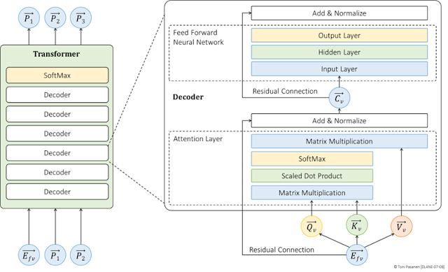
The Transformer consists of stacks of decoder modules. A word embedding vector, a result of the word tokenization and embbeding, is fed as input to the first decoder module. After processing, the resulting context vector is passed to the next decodeer, and so on. After the final decoder, a softmax layer evaluates the output against the complete vocabulary to predict the next word. As an autoregressive model, the predicted word vector from the softmax layer is converted into a token before being fed back into the subsequent decoder layer. This process involves a token-to-word vector transformation prior to re-entering the decoder.

Each decoder module consists of an attention layer, Add & Normalization layer and a feedforward neural network (FFNN). Rather than feeding the embedded word vector (i.e., token embedding plus positional encoding) directly into the decoder layers, the Transformer first computes the Query (Q), Key (K), and Value (V) vectors from the word vector. These vectors are then used in the self-attention mechanism. Initially, the query vector is multiplied by the key vectors using matrix multiplication. The result is then divided by the square root of the dimension of the key vectors (scaled dot product) to obtain the logits. The logits are processed by a softmax layer to compute probabilities. The SoftMax prediction results are multiplied with the value vectors to produce a context vector.

Before feeding the context vector into the feedforward neural network, it is summed with the original word embedding vector (which includes positional encoding) via a residual connection. Finally, the output is normalized using layer normalization. This normalized output is then passed as input to the FFNN, which computes the output. 

The basic architecture of the FFNN in the decoder is designed so that the input layer has as many neurons as the dimension of the context vector. The hidden layer, in turn, has four times as many neurons as the input layer, while the output layer has the same number of neurons as the input layer. This design guarantees that the output vector of the FFNN has the same dimension as the context vector. Like the attention block, the FFNN block also employs residual connections and normalization.

Figure 7-8: Decoder-Only Transformer Architecture.

Query, Key and Value Vectors

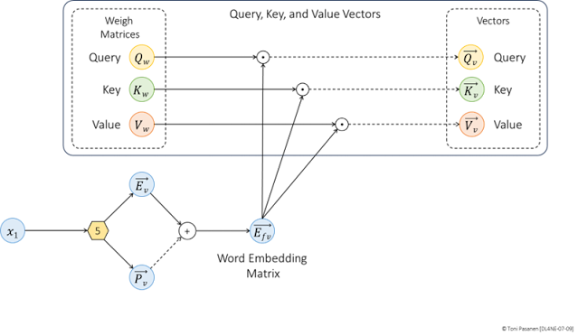
As pointed out in the Introduction, the word embedding vector is not used as input to the first decoder. Instead, it is multiplied by pretrained Query, Key, and Value weight matrices. The result of this matrix multiplication, dot product, produces the Query, Key, and Value vectors, which are use as inputs, and are processed through the Transformer. Figure 7–9 show the basic workflow of this process.

Figure 7-9: Query, Key, and Value Vectors.

Let’s take a closer look at the process using numbers. After tokenizing the input words and applying positional encoding, we obtain a final 5-dimensional word matrix. To reduce computation cycles, the process reduces the dimension of the Query vector from 5 to 3. Because we want the Query vector to be three-dimensional, we use three 5-dimensional column vectors, each of which is multiplied by the word vector.

Figure 7-10: Calculating the Query Vector.

Figure 7–11 depicts the calculation process, where each component of the word vector is multiplied by its corresponding component in the Query weight matrix. The weighted sum of these results forms a three-dimensional Query vector. The Key and Value vectors are calculated using the same method.

The same Query, Key, and Value (Q, K, V) weight matrices are used across all words (tokens) within a single self-attention layer in a Transformer model. This ensures that each token is processed in the same way, maintaining consistency in the attention computations. However, each decoder layer in the Transformer has its own dedicated Q, K, and V weight matrices, meaning that every layer learns different transformations of the input tokens, allowing deeper layers to capture more abstract representations.

Figure 7-11: Calculating the Query Vector.

Attention Layer

Figure 7-12 depicts what happens in the first three components of the Attention layer after calculating the Query, Key, and Value vectors. In this example, we focus on the word “clear”, and try to predict the next word. Its Query vector is multiplied by its own Key vector as well as by all the Key vectors generated for the preceding words. Each multiplication produces its own score. Note that the score values shown in the figure are theoretical and are not derived from the actual Qv × Kv matrix multiplication; however, the remaining values are based on these calculations. Additionally, in our example, we use one-dimensional values (instead of actual vectors) to keep the figures and calculations simple. In reality, these are n-dimensional vectors.

After the Qv × Kv matrix multiplication, the resulting scores are divided by the square root of the vector depth, yielding logits, i.e., the input values for the softmax function. The softmax function then computes the exponential of each logit (using Euler’s number, approximately 2.71828) and divides each result by the sum of all exponentials. For example, the value 3.16, corresponding to the first word, is divided by 482.22, resulting in a probability of 0.007. Note that the sum of the probabilities is 1.0. Softmax ensures that the attention scores sum to 1, making them interpretable as probabilities and helping the model decide which input tokens to focus on when generating an output. In our example, the token for the word “clear” has the highest probability at this stage. The word “decided” has the second highest probability score (0.210), which indicates that the semantics of “clear”, which has the highest probability score (0.665), can be interpreted as an verb answering the question: “What she decided to do?

Figure 7-12: Attention Layer, the First Three Steps.

Next, the SoftMax probabilities are multiplied by each token's Value vector (matrix multiplication). The resulting vectors are then summed, producing the Context vector for the token associated with the word “clear.” Note that the components of the Value vectors are example values and are not derived from actual computations.

Figure 7-13: Attention Layer, the Fourth Step.

Add & Normalization

As the final step, the Word vector, which includes positional encoding, is added to the context vector via a Residual Connection. The result is then passed through a normalization process, where the vector’s components are summed and divided by the vector’s dimension, yielding the mean (μ). This mean value is then used for standard deviation calculation: the mean is subtracted from each of the three vector components, and the results are squared. These squared values are then summed, divided by three (the vector’s dimension), and the square root of this result gives the final output vector [1.40, -0.55, -0.87] of the Add & Normalize layer. 

Figure 7-14: Add & Normalize Layer – Residual Connection and Layer Normalization.

Feed Forward Neural Network

Within the decoder module, the feedforward neural network uses the output vector from the Add & Normalize layer as its input. In our example, the FFNN have one neuron in input layer for each component of the vector. This layer simply passes the input values to the hidden layer, where each neuron first calculates a weighted sum and then applies the ReLU activation function. In our example, the hidden layer contains nine neurons (three times the number of input neurons). The output from the hidden layer is then fed to the output layer, where the neurons again compute a weighted sum and apply the ReLU activation function. Note that in transformer-based decoders, the FFNN is applied to each token individually. This means that each token-related output from the attention layer is processed separately by the same FFNN model with shared weights, ensuring a consistent transformation of each token's representation regardless of its position in the sequence.

Figure 7-15: Fully Connected Feed Forward Neural Network (FFNN).

The final decoder output is computed in the Add & Normalize layer, similarly as Add & Normalize after the attention layer. This produces the decoder output, which is used as the input for the next decoder module. 

Figure 7-16: Add & Normalize Layer – Residual Connection and Layer Normalization.

Next Word Probability Computation – SoftMax Function

The output of the last decoder module does not directly represent the next word. Instead, it must be transformed into a probability distribution over the entire vocabulary. First, the decoder output is passed through a weight matrix that maps it to a new vector, where each element corresponds to a word in the vocabulary. For example, in Figure 7-17 the vocabulary consists of 12 words. These words are tokenized and linked to their corresponding word embeddings vector. That said, the word embedding matrix serves as a weight matrix.

Figure 7-17: Hidden State Vector and Word Embedding Matrix.

Figure 7-18 illustrates how the decoder output vector (i.e., the hidden state h) is multiplied by all word embedding vectors to produce a new vector of logits. 

Figure 7-18: Logits Calculation – Dot Product of Hidden State and Complete Vocabulary.

Next, the SoftMax function is applied to the logits. This function converts the logits into probabilities by exponentiating each logit and then normalizing by the sum of all exponentiated logits. The result is a probability distribution in which each value represents the likelihood of selecting a particular word as the next token.

Figure 7-19: Probability Calculation - Adding Logits to SoftMax Function

Finally, the word with the highest probability is selected as the next token. This token is then mapped back to its corresponding word using a token-to-word lookup. This initiates the next iteration, where the token is converted into its word embedding vector, and used together with positional encoding to create the actual word embedding for the next iteration.

Figure 7-20: Word-to-Token, and Token-to-Word Embedding Process.

In theory, our simple example shows that the model can assign the highest probability to the correct word. For instance, by analyzing the position of the word “clear” relative to its preceding words, the model is able to infer the context. When the context implies that an action is directed toward a known target, the article “the” receives the highest probability score and is predicted as the next word.

Conclusion

We use pretty simple examples in this chapter. However, GPT-3, for example, is built on a deep Transformer architecture comprising 96 decoder blocks. Each decoder block is divided into three primary sub-layers:

Attention Layer: This layer implements multi-head self-attention using four key weight matrices, one each for the query, key, and value projections, plus one for the output projection. Together, these matrices account for roughly 600 million trainable parameters per block.

Add & Normalize Layers: Each block employs two residual connections paired with layer normalization. The first Add & Normalize operation occurs immediately after the Attention Layer, and the second follows the Feed-Forward Neural Network (FFNN) layer. Although essential for stabilizing training, the parameters in each normalization step are relatively few, typically on the order of tens of thousands.

Feed-Forward Neural Network (FFNN) Layer: The FFNN consists of two linear transformations with an intermediate expansion (usually about four times the model’s hidden size). This layer contributes approximately 1.2 billion parameters per block.

Aggregating the parameters from all 96 decoder blocks, and including additional parameters from the token embeddings, positional encodings, and other components, the entire GPT-3 model totals around 175 billion trainable parameters. This is why parallelism is essential: the training process must be distributed across multiple GPUs and executed according to a selected parallelization strategy. The second part of the book discusses about Parallelization.

Large Language Models (LLM) - Part 1/2: Word Embedding

Introduction

This chapter introduces the basic operations of Transformer-based Large Language Models (LLMs), focusing on fundamental concepts rather than any specific LLM, such as OpenAI’s GPT (Generative Pretrained Transformer).The chapter begins with an introduction to tokenization and word embeddings, which convert input words into a format the model can process. Next, it explains how the transformer component leverages decoder architecture for input processing and prediction. 

This chapter has two main goals. First, it explains how an LLM understands the context of a word. For example, the word “clear” can be used as a verb (Please, clear the table.) or as an adjective (The sky was clear.), depending on the context. Second, it discusses why LLMs require parallelization across hundreds or even thousands of GPUs due to the large model size, massive datasets, and the computational complexity involved.

Tokenizer and Word Embedding Matrix

As a first step, we import a vocabulary into the model. The vocabulary used for training large language models (LLMs) typically consists of a mix of general and domain-specific terms, including basic vocabulary, technical terminology, academic and formal language, idiomatic expressions, cultural references, as well as synonyms and antonyms. Each word and character is stored in a word lookup table and assigned a unique token. This process is called tokenization.

Many LLMs use Byte Pair Encoding (BPE), which splits words into subword units. For example, the word "unhappiness" might be broken down into "un," "happi," and "ness." BPE is widely used because it effectively balances vocabulary size and tokenization efficiency, particularly for handling rare words and sub-words. For simplicity, we use complete words in all our examples.

Figure 7-1 illustrates the relationship between words in the vocabulary and their corresponding tokens. Token values start from 2 because token 0 is reserved for padding and token 1 for unknown words.

Each token, representing a word, is mapped to a Word Embedding Vector, which is initially assigned random values. The collection of these vectors forms a Word Embedding Matrix. The dimensionality of each vector determines how much contextual information it can encode.

For example, consider the word “clear.” A two-dimensional vector may distinguish it as either an adjective or a verb but lacks further contextual information. By increasing the number of dimensions, the model can capture more context and better understand the meaning of the word. In the sentence “The sky was clear,” the phrase “The sky was” suggests that "clear" is an adjective. However, if we extend the sentence to “She decided to clear the backyard of junk,” the word "clear" now functions as a verb. More dimensions allow the model to utilize surrounding words more effectively for next-word prediction. For instance, GPT-3 uses 12,288-dimensional vectors. Given a vocabulary size of 50,000 words used by GPT-3, the Word Embedding Matrix has dimensions of 12,288 × 50,000, resulting in 614,400,000 parameters.

The context size, defined as the sequence length of vectors, determines how many preceding words the model considers when predicting the next word. In GPT-3, the context size is 2,048 tokens.

Figure 7-1: Tokenization and Word Embedding Matrix.

 

Word Embedding

As a first step, when we feed input words into a Natural Language Processing (NLP) model, we must convert them into a format the model can understand. This is a two-step process:

1. Tokenization – Each word is assigned a corresponding token from a lookup table.
2. Word Embedding – These token IDs are then mapped to vectors using a word embedding lookup table.

To keep things simple, Figure 7-2 uses two-dimensional vectors in the embedding matrix. Instead of complete sentences, we use words, which can be categorized into four groups: female, male, adult, and child.

The first word, "Wife," appears in the lookup table with the token value 2. The corresponding word vector in the lookup table for token 2 is [-4.5, -3.0]. Note that Figure 7-2 represents vectors as column vectors, whereas in the text, I use row vectors—but they contain the same values.

The second word, "Mother," is assigned the token 3, which is associated with the word vector [-2.5, +3.0], and so on.

Figure 7-2: Word Tokenization and Word Embedding.

In Figure 7-3, we have a two-dimensional vector space divided into four quadrants, representing gender (male/female) and age (child/adult). Tokenized words are mapped into this space.

At the start of the first iteration, all words are placed randomly within the two-dimensional space. During training, our goal is to adjust the word vector values so that adults are positioned on the positive side of the Y-axis and children on the negative side. Similarly, males are placed in the negative space of the X-axis, while females are positioned on the positive side.

Figure 7-3: Words in the 2 Dimensional Vector Space in the Initial State.

Figure 7-4 illustrates how words may be positioned after successful training. All words representing a male adult are placed in the upper-left quadrant (adult/male). Similarly, all other words are positioned in the two-dimensional vector space based on their corresponding age and gender.

Figure 7-4: Words in the 2 Dimensional Vector Space After Training.

In addition to grouping similar words, such as "adult/female," close to each other in an n-dimensional space, there should also be positional similarities between words in different quadrants. For example, if we calculate the Euclidean distance between the words Father and Mother, we might find that their distance is approximately 4.3. The same pattern applies to word pairs like Nephew-Niece, Brother-Sister, Husband-Wife, and Father-in-Law–Mother-in-Law.

However, it is important to note that this example is purely theoretical. In practice, Euclidean distances in high-dimensional word embeddings are not fixed but vary depending on the training data and optimization process. The relationships between words are often better captured through cosine similarity rather than absolute Euclidean distances.

Figure 7-5: Euclidean Distance.

Positional Embeddings

Since input text often contains repeated words with different meanings depending on their position, an LLM must distinguish between them. To achieve this, the word embedding process in Natural Language Processing (NLP) incorporates a Positional Encoding Vector alongside the Word Embedding Vector, resulting in the final word representation.

In Figure 7-6, the sentence "The sky is clear, so she finally decided to clear the backyard" contains the word clear twice. Repeated words share the same token ID instead of receiving unique ones. In this example, the is assigned token ID 2, and clear is assigned 5. These token IDs are then mapped to vectors using a word embedding lookup table. However, without positional encoding, words with different meanings would share the same vector representation.

Focusing on clear (token ID 5), it maps to the word embedding vector [+2.5, +1.0] from the lookup table. Since token IDs do not capture word position, identical words always receive the same embedding.

Positional encoding is essential for capturing context and semantic meaning. As shown in Figure 7-6, each input word receives a Positional Encoding Vector (PE) in addition to its word embedding. PE can either be learned and adjusted during training or remain fixed. The final Word Embedding Vector is computed by combining both the Word Embedding Vector and Positional Encoding Vector.

Figure 7-6: Tokenization – Positional Embedding Vector.

Calculating the Final Word Embedding

Figure 7-2 presents the equations for computing the final word embedding by incorporating positional embeddings. There are three variables:

• Position (pos) → The word’s position in the sentence. In our example, the first occurrence of clear is the fourth word, so pos = 4.
• Dimension (d) → The depth of the vector. We use a 2-dimensional vector, so d = 2.
• Index (i) → Specifies the axis of the vector: 0 for the x-axis and 1 for the y-axis.

The positional embedding is computed using the following equations:

• x-axis: sin(pos/100002i/d), where i = 0
• y-axis: cos(pos/100002i/d, where i = 1

For clear at position 4, with d = 2, the resulting 2D positional vector is [-0.8, +1.0]. This vector is then added to the input word embedding vector [+2.5, +1.0], resulting in the final word embedding vector [+1.7, +2.0].

Figure 7-7 also shows the final word embedding for the second occurrence of clear, but the computation is omitted.

Figure 7-7: Finals Word Embedding for the 4th Word.